Instructor: Lingqi Yan | UCSB Bilibili: https://www.bilibili.com/video/BV1X7411F744
1 Why Study Transformations
Transformations have two core applications in graphics:
| Application | Description | Example |
|---|---|---|
| Modeling | Place objects in a scene | Translate, rotate, scale objects |
| Viewing | Project 3D scene onto a 2D image | Camera transform, projection transform |
2 2D Transformations
Scale
Uniform scale (all directions scaled equally):
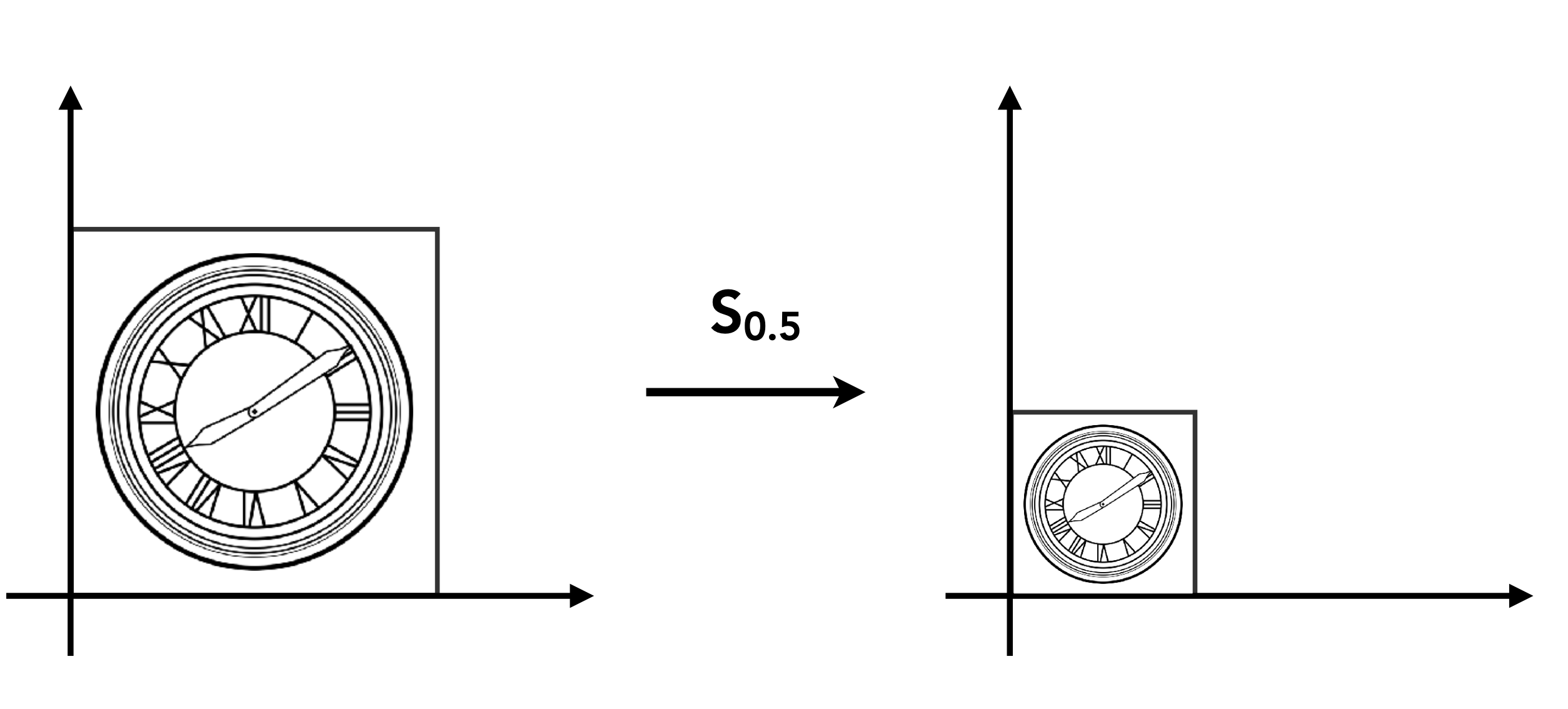
$x' = sx \qquad y' = sy$
$$ \begin{pmatrix} x' \\ y' \end{pmatrix} = \begin{pmatrix} s & 0 \\ 0 & s \end{pmatrix} \begin{pmatrix} x \\ y \end{pmatrix} $$For example: $x = 2, \; y = 2, \; s = 0.5$
$$ \begin{pmatrix} x' \\ y' \end{pmatrix} = \begin{pmatrix} 0.5 & 0 \\ 0 & 0.5 \end{pmatrix} \begin{pmatrix} 2 \\ 2 \end{pmatrix} = \begin{pmatrix} 0.5 \times 2 + 0 \times 2 \\ 0 \times 2 + 0.5 \times 2 \end{pmatrix} = \begin{pmatrix} 1 \\ 1 \end{pmatrix} $$Non-uniform scale (each direction scaled independently):
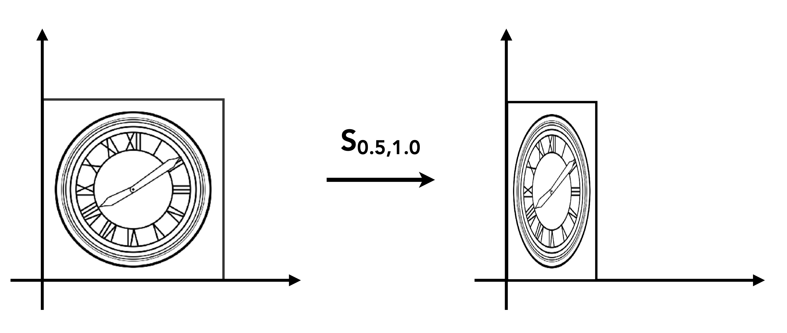
Reflection

Reflection about the y-axis:
$$ \begin{pmatrix} x' \\ y' \end{pmatrix} = \begin{pmatrix} -1 & 0 \\ 0 & 1 \end{pmatrix} \begin{pmatrix} x \\ y \end{pmatrix} = \begin{pmatrix} -x \\ y \end{pmatrix} $$Shear
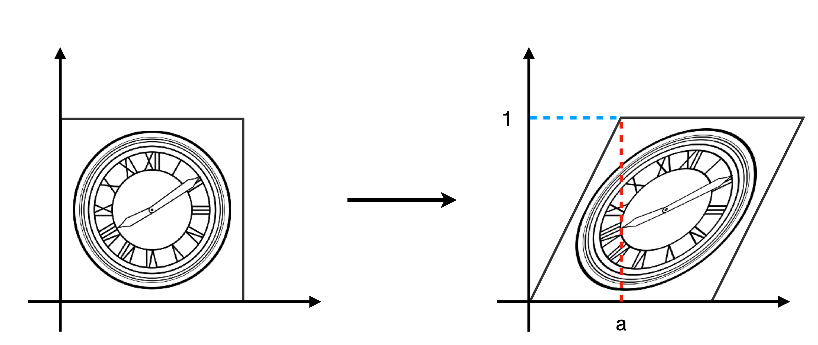
Horizontal shear (y=0 stays fixed, y=1 shifts horizontally by a):
$$ \begin{pmatrix} x' \\ y' \end{pmatrix} = \begin{pmatrix} 1 & a \\ 0 & 1 \end{pmatrix} \begin{pmatrix} x \\ y \end{pmatrix} $$The parameter $a$ controls the tilt. When $a = 0$ the matrix reduces to the identity (no transform); the larger $a$, the more obvious the tilt.
Rotation
The default rotation origin is $(0, 0)$, counterclockwise is the positive direction, and the rotation angle is $\theta$.
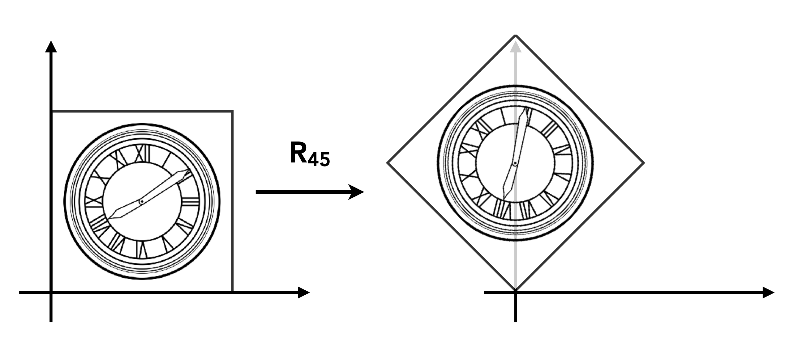
Rotate by $\theta$ counterclockwise about the origin:
$$ \begin{pmatrix} x' \\ y' \end{pmatrix} = \begin{pmatrix} \cos\theta & -\sin\theta \\ \sin\theta & \cos\theta \end{pmatrix} \begin{pmatrix} x \\ y \end{pmatrix} $$Denoted as $R_\theta$. Special cases:
- $R_{90°} = \begin{pmatrix} 0 & -1 \\ 1 & 0 \end{pmatrix}$
- $R_{-90°} = \begin{pmatrix} 0 & 1 \\ -1 & 0 \end{pmatrix}$

Deriving the Rotation Formula
Let the rotation matrix be unknown $R = \begin{pmatrix} A & B \\ C & D \end{pmatrix}$. Given the results of rotating the two basis vectors, substitute and solve. Assuming the square has side length 1, we can derive the coordinates of the four points and side lengths.
Basis vector $e_1 = (1, 0)$ after rotating by $\theta$ → $(\cos\theta, \sin\theta)$:
$$ \begin{pmatrix} A & B \\ C & D \end{pmatrix} \begin{pmatrix} 1 \\ 0 \end{pmatrix} = \begin{pmatrix} A \times 1 + B \times 0 \\ C \times 1 + D \times 0 \end{pmatrix} = \begin{pmatrix} A \\ C \end{pmatrix} = \begin{pmatrix} \cos\theta \\ \sin\theta \end{pmatrix} \implies A = \cos\theta, \; C = \sin\theta $$Basis vector $e_2 = (0, 1)$ after rotating by $\theta$ → $(-\sin\theta, \cos\theta)$:
$$ \begin{pmatrix} A & B \\ C & D \end{pmatrix} \begin{pmatrix} 0 \\ 1 \end{pmatrix} = \begin{pmatrix} A \times 0 + B \times 1 \\ C \times 0 + D \times 1 \end{pmatrix} = \begin{pmatrix} B \\ D \end{pmatrix} = \begin{pmatrix} -\sin\theta \\ \cos\theta \end{pmatrix} \implies B = -\sin\theta, \; D = \cos\theta $$The rotation matrix:
$$ R_\theta = \begin{pmatrix} \cos\theta & -\sin\theta \\ \sin\theta & \cos\theta \end{pmatrix} $$Expanding the rotation of an arbitrary point $(x, y)$:
$$ \begin{pmatrix} x' \\ y' \end{pmatrix} = \begin{pmatrix} \cos\theta & -\sin\theta \\ \sin\theta & \cos\theta \end{pmatrix} \begin{pmatrix} x \\ y \end{pmatrix} = \begin{pmatrix} x\cos\theta - y\sin\theta \\ x\sin\theta + y\cos\theta \end{pmatrix} $$Unified Representation of Linear Transforms
All 2D linear transforms can be represented by matrix multiplication:
$$ \begin{pmatrix} x' \\ y' \end{pmatrix} = \begin{pmatrix} a & b \\ c & d \end{pmatrix} \begin{pmatrix} x \\ y \end{pmatrix} $$That is, $x' = M x$.
3 Homogeneous Coordinates
Why Do We Need Homogeneous Coordinates
Problem: Translation is not a linear transform, so it cannot be represented by a 2×2 matrix!
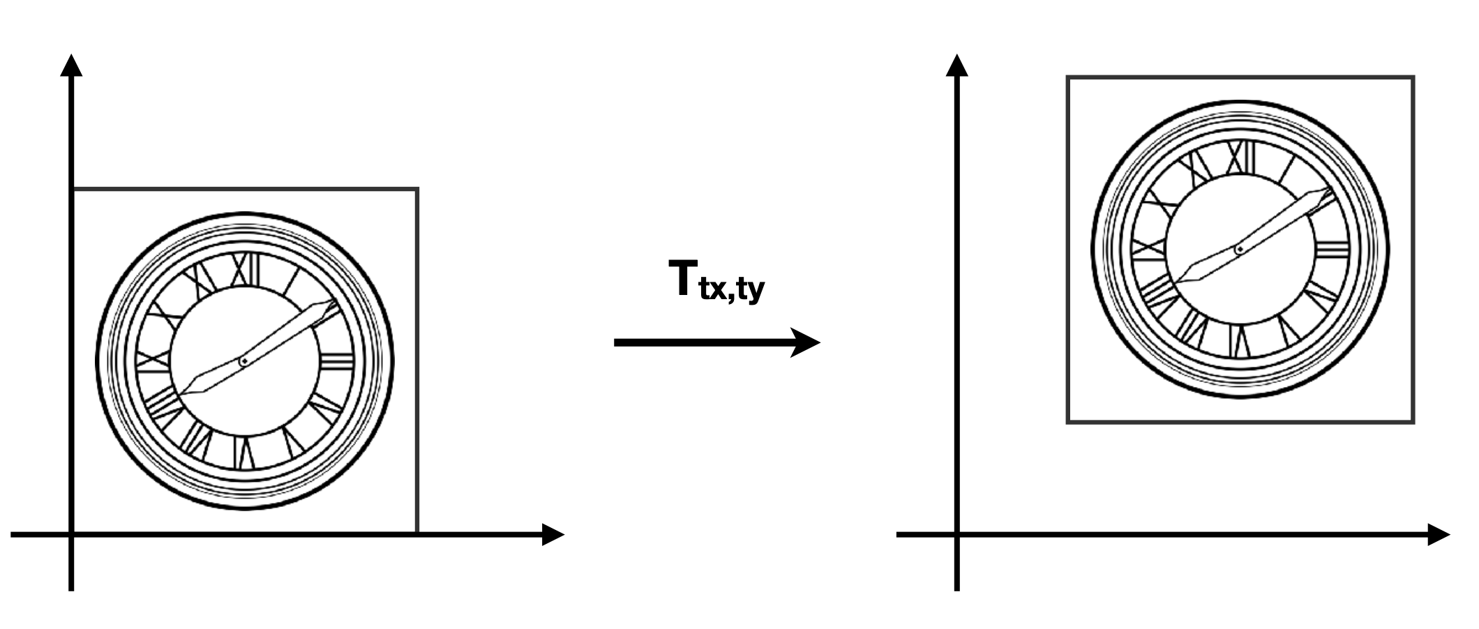
$x' = x+t_x \qquad y' = y+t_y$
$$ \begin{pmatrix} x' \\ y' \end{pmatrix} = \begin{pmatrix} a & b \\ c & d \end{pmatrix} \begin{pmatrix} x \\ y \end{pmatrix} + \begin{pmatrix} t_x \\ t_y \end{pmatrix} $$We want a unified matrix form to represent all affine transforms (linear transform + translation).
Definition of Homogeneous Coordinates
Add a third coordinate (the w coordinate):
| Type | Homogeneous representation | Explanation |
|---|---|---|
| 2D point | $(x, y, 1)^T$ | A point has a position → needs translation → w = 1 |
| 2D vector | $(x, y, 0)^T$ | A vector has no position (direction only) → no translation → w = 0 |
Matrix representation of translation:
$$ \begin{pmatrix} x' \\ y' \\ w' \end{pmatrix} = \begin{pmatrix} 1 & 0 & t_x \\ 0 & 1 & t_y \\ 0 & 0 & 1 \end{pmatrix} \begin{pmatrix} x \\ y \\ 1 \end{pmatrix} = \begin{pmatrix} 1 \times x + 0 \times y + t_x \times 1 \\ 0 \times x + 1 \times y + t_y \times 1 \\ 0 \times x + 0 \times y + 1 \times 1 \end{pmatrix} = \begin{pmatrix} x + t_x \\ y + t_y \\ 1 \end{pmatrix} $$Key property: $(x, y, w)^T$ represents the 2D point $(x/w, y/w)^T$ (when $w \neq 0$).
For example: $(1, 0, 1)$ and $(2, 0, 2)$ represent the same point $(1, 0)$.
Operations in Homogeneous Coordinates
Validity check: an operation is valid if the resulting w coordinate is 1 or 0:
- vector + vector = vector
- point − point = vector
- point + vector = point
- point + point = ?? (w = 2, invalid → divide by w to normalize)
Restoring a point: $\begin{pmatrix} x \\ y \\ w \end{pmatrix}$ corresponds to the 2D point $\begin{pmatrix} x/w \\ y/w \\ 1 \end{pmatrix}$, where $w \neq 0$.
| w value | Meaning | Transform behavior | |
|---|---|---|---|
| Point | 1 | Has a position | Accepts rotation, scale, translation |
| Vector | 0 | No position | Accepts rotation, scale, ignores translation |
4 Affine Transformation
Definition
Affine transformation = linear transformation + translation
$$ \begin{pmatrix} x' \\ y' \end{pmatrix} = \begin{pmatrix} a & b \\ c & d \end{pmatrix} \cdot \begin{pmatrix} x \\ y \end{pmatrix} + \begin{pmatrix} t_x \\ t_y \end{pmatrix} $$Unified Representation in Homogeneous Coordinates
$$ \begin{pmatrix} x' \\ y' \\ 1 \end{pmatrix} = \begin{pmatrix} a & b & t_x \\ c & d & t_y \\ 0 & 0 & 1 \end{pmatrix} \cdot \begin{pmatrix} x \\ y \\ 1 \end{pmatrix} $$Summary of 2D Transform Matrices in Homogeneous Coordinates
| Transform | Homogeneous matrix |
|---|---|
| Translation | $T(t_x, t_y) = \begin{pmatrix} 1 & 0 & t_x \\ 0 & 1 & t_y \\ 0 & 0 & 1 \end{pmatrix}$ |
| Scale | $S(s_x, s_y) = \begin{pmatrix} s_x & 0 & 0 \\ 0 & s_y & 0 \\ 0 & 0 & 1 \end{pmatrix}$ |
| Rotation | $R(\theta) = \begin{pmatrix} \cos\theta & -\sin\theta & 0 \\ \sin\theta & \cos\theta & 0 \\ 0 & 0 & 1 \end{pmatrix}$ |
5 Inverse Transform
An inverse transform “undoes” a transform.
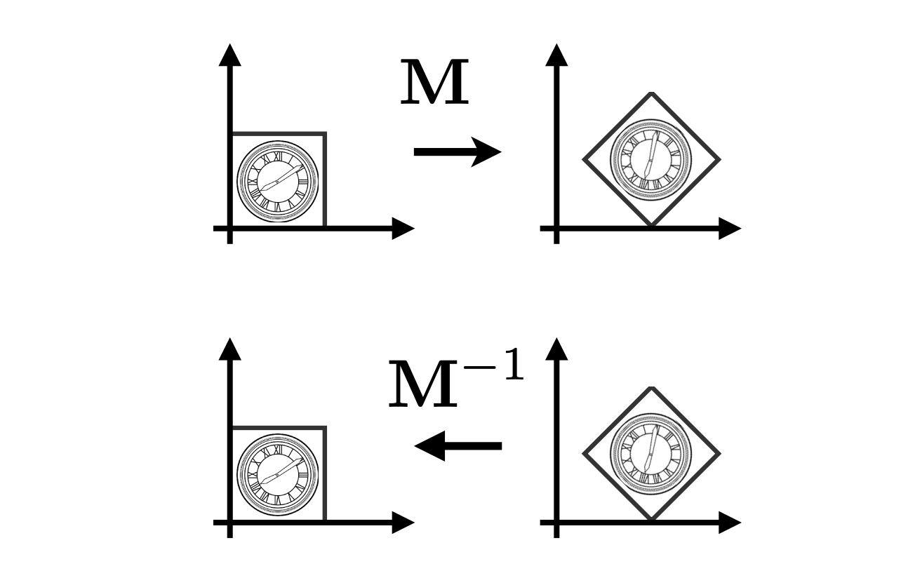
The inverse matrix $M^{-1}$ of a transform matrix $M$ represents the reverse transform:
- Translation $T^{-1}(t_x, t_y) = T(-t_x, -t_y)$
- Rotation $R^{-1}(\theta) = R(-\theta) = R^T(\theta)$ (for orthogonal matrices, the inverse equals the transpose)
- Scale $S^{-1}(s_x, s_y) = S(1/s_x, 1/s_y)$
6 Composing Transforms
Order Matters!

Matrix multiplication is not commutative:
$$ R_{45°} \cdot T_{(1,0)} \neq T_{(1,0)} \cdot R_{45°} $$Matrices are applied right to left (the one written first is applied first):
$$ T_{(1,0)} \cdot R_{45°} \begin{pmatrix} x \\ y \\ 1 \end{pmatrix} = \begin{pmatrix} 1 & 0 & 1 \\ 0 & 1 & 0 \\ 0 & 0 & 1 \end{pmatrix}\begin{pmatrix} \cos{45°} & -\sin{45°} & 0 \\ \sin{45°} & \cos{45°} & 0 \\ 0 & 0 & 1 \end{pmatrix}\begin{pmatrix} x \\ y \\ 1 \end{pmatrix} $$This means: rotate by 45° first, then translate by (1,0).
Combining Transforms
Multiple transforms can be combined into a single matrix via matrix multiplication:
$$ A_n(...A_2(A_1(\vec{x}))) = A_n \cdots A_2 \cdot A_1 \cdot \begin{pmatrix} x \\ y \\ 1 \end{pmatrix} $$Pre-multiplying n matrices yields a single matrix representing the combined transform, which is very important for performance and yields the rotation-translation matrix.
Rotation about an Arbitrary Point
How to rotate about a given point $c$?
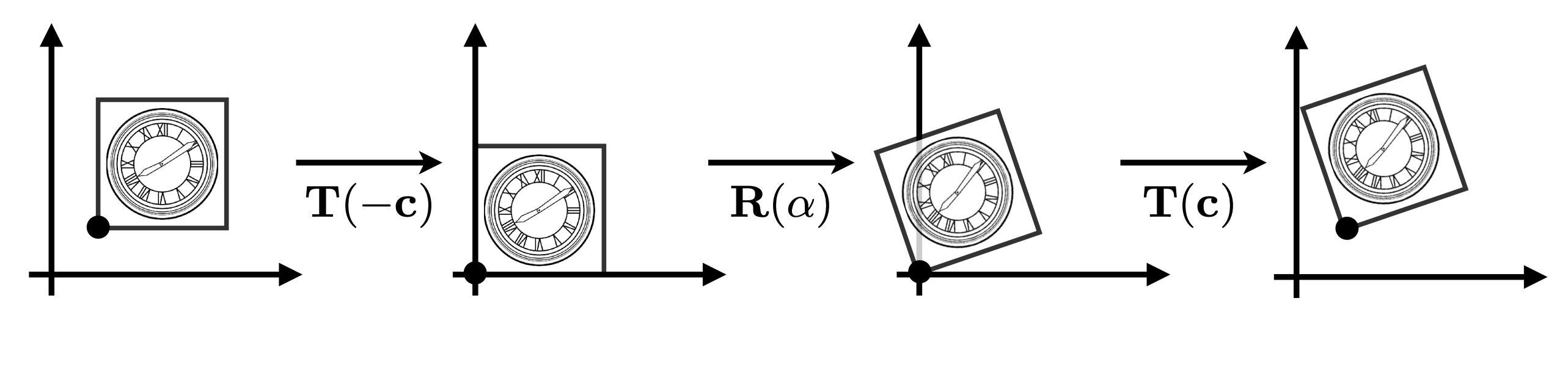
- Translate: move the rotation center $c$ to the origin → $T(-c)$
- Rotate: rotate about the origin → $R(\alpha)$
- Translate: move back → $T(c)$
7 3D Transformations
Homogeneous Coordinate Representation
- 3D point: $(x, y, z, 1)^T$
- 3D vector: $(x, y, z, 0)^T$
- In general, $(x, y, z, w)^T$ ($w \neq 0$) represents the 3D point $(x/w, y/w, z/w)$
Use 4×4 matrices for affine transforms:
$$ \begin{pmatrix} x' \\ y' \\ z' \\ 1 \end{pmatrix} = \begin{pmatrix} a & b & c & t_x \\ d & e & f & t_y \\ g & h & i & t_z \\ 0 & 0 & 0 & 1 \end{pmatrix} \cdot \begin{pmatrix} x \\ y \\ z \\ 1 \end{pmatrix} $$Properties of the Rotation Matrix
$\cos\theta$ is a symmetric curve, so $\cos\theta$ and $\cos(-\theta)$ are equal; $\sin\theta$ is an antisymmetric curve, so $\sin\theta$ and $\sin(-\theta)$ are opposites. From this:
$$ R(-\theta) = \begin{pmatrix} \cos\theta & \sin\theta \\ -\sin\theta & \cos\theta \end{pmatrix} = R(\theta)^T $$The rows of $R(-\theta)$ equal the columns of $R(\theta)$, and they are inverse matrices:
$$ R(-\theta) = R(\theta)^{-1} \quad \text{(by definition)} $$Mathematically, a matrix whose inverse equals its transpose is an orthogonal matrix; rotation matrices are orthogonal matrices.
3D Transform Matrices
Scale:
$$ S(s_x, s_y, s_z) = \begin{pmatrix} s_x & 0 & 0 & 0 \\ 0 & s_y & 0 & 0 \\ 0 & 0 & s_z & 0 \\ 0 & 0 & 0 & 1 \end{pmatrix} $$Translation:
$$ T(t_x, t_y, t_z) = \begin{pmatrix} 1 & 0 & 0 & t_x \\ 0 & 1 & 0 & t_y \\ 0 & 0 & 1 & t_z \\ 0 & 0 & 0 & 1 \end{pmatrix} $$Rotation about the coordinate axes:
Rotation about the x-axis:
$$ R_x(\alpha) = \begin{pmatrix} 1 & 0 & 0 & 0 \\ 0 & \cos\alpha & -\sin\alpha & 0 \\ 0 & \sin\alpha & \cos\alpha & 0 \\ 0 & 0 & 0 & 1 \end{pmatrix} $$Rotation about the y-axis (note the direction):
$$ R_y(\alpha) = \begin{pmatrix} \cos\alpha & 0 & \sin\alpha & 0 \\ 0 & 1 & 0 & 0 \\ -\sin\alpha & 0 & \cos\alpha & 0 \\ 0 & 0 & 0 & 1 \end{pmatrix} $$Rotation about the z-axis:
$$ R_z(\alpha) = \begin{pmatrix} \cos\alpha & -\sin\alpha & 0 & 0 \\ \sin\alpha & \cos\alpha & 0 & 0 \\ 0 & 0 & 1 & 0 \\ 0 & 0 & 0 & 1 \end{pmatrix} $$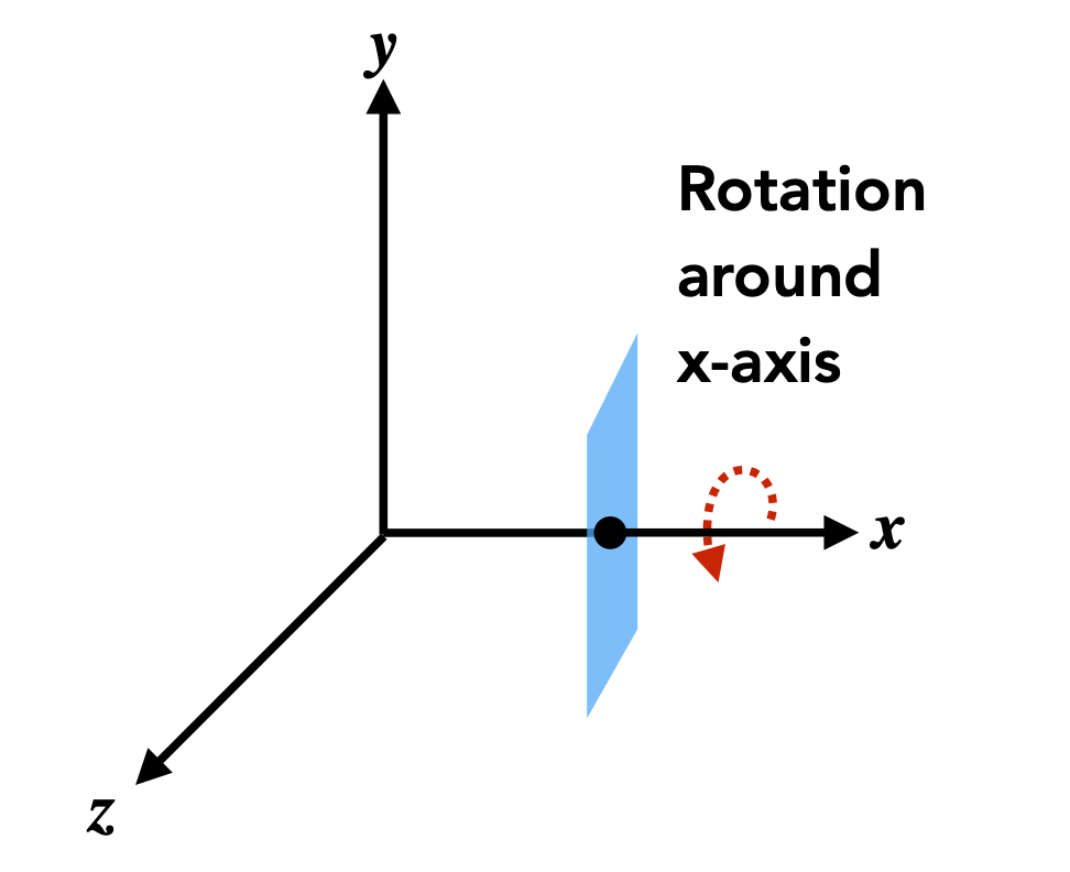
Euler Angles
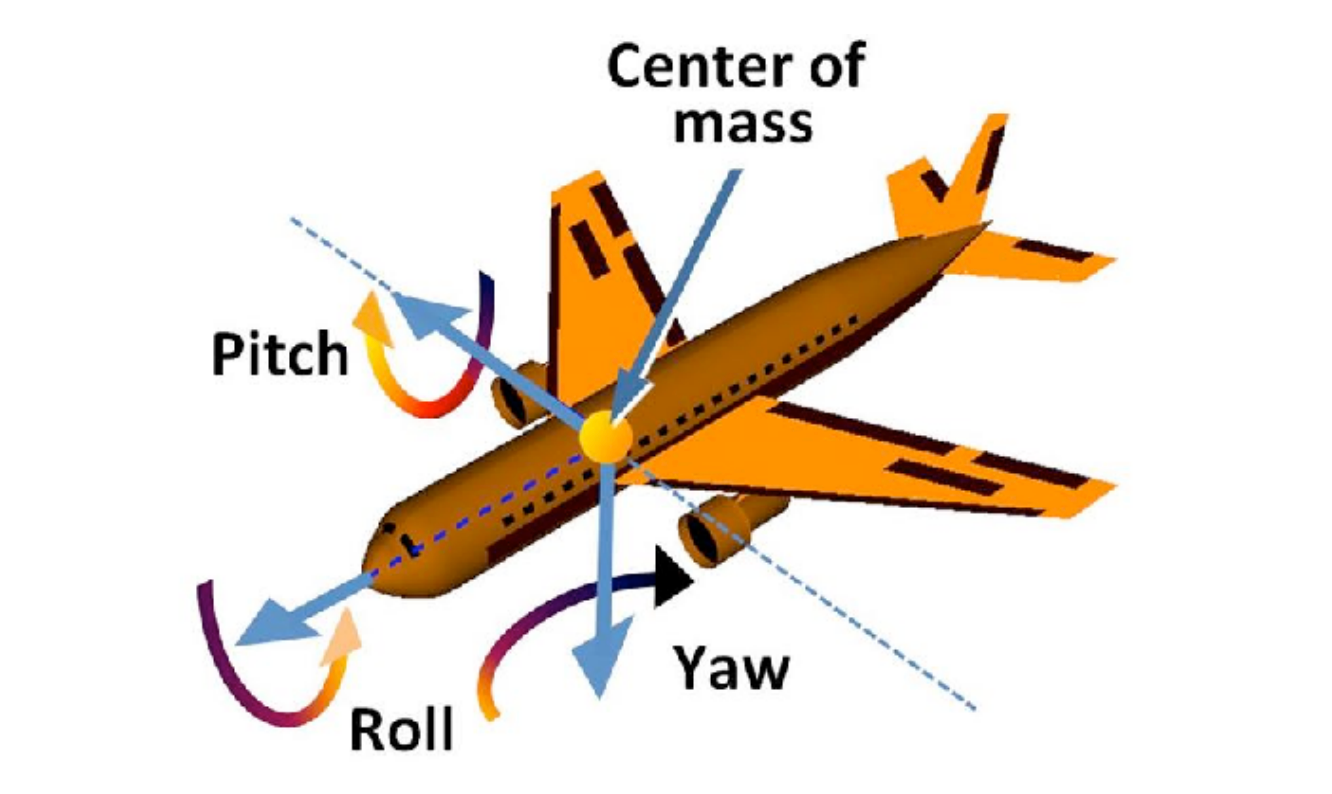
Any 3D rotation can be represented by combining rotations about the three axes:
$$ R_{xyz}(\alpha, \beta, \gamma) = R_x(\alpha) \cdot R_y(\beta) \cdot R_z(\gamma) $$Commonly used in flight simulators: Roll, Pitch, Yaw.
Rodrigues’ Rotation Formula
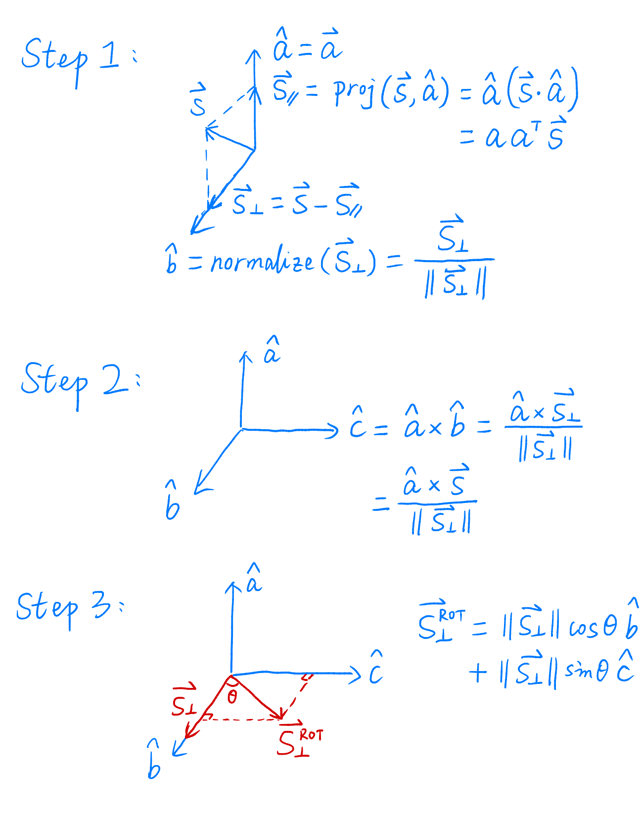
Rotating by $\alpha$ about an arbitrary unit axis $\vec{n}$:
$$ R(\vec{n}, \alpha) = \cos\alpha \cdot I + (1 - \cos\alpha) \vec{n} \vec{n}^T + \sin\alpha \cdot N $$where $N$ is the cross-product matrix:
$$ N = \begin{pmatrix} 0 & -n_z & n_y \\ n_z & 0 & -n_x \\ -n_y & n_x & 0 \end{pmatrix} $$Derivation: see the course supplementary material.
8 MVP Transform Overview
The three major transforms in the graphics rendering pipeline:
Model coords → [Model] → World coords → [View] → Camera coords → [Projection] → Clip coords
| Transform | Function | Description |
|---|---|---|
| Model | Model coords → World coords | Place objects in a scene |
| View | World coords → Camera coords | Determine the viewing angle |
| Projection | Camera coords → Clip coords | 3D → 2D projection |
9 View Transformation
Analogy to Taking a Photo
- Position and arrange people → Model transform
- Find an angle, place the camera → View transform
- Press the shutter → Projection transform
Camera Definition
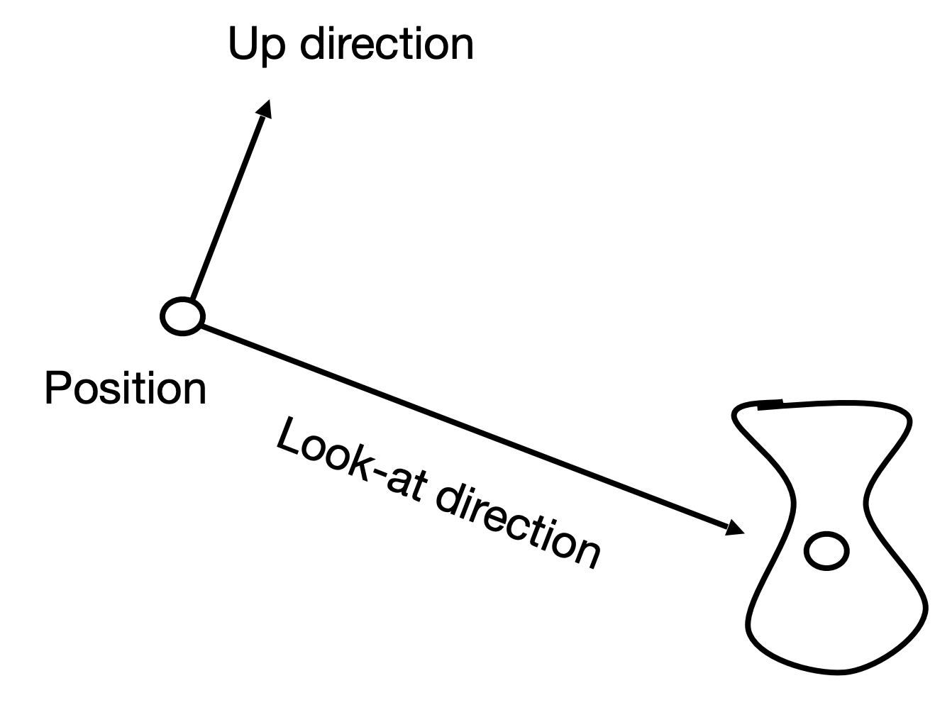
| Parameter | Symbol | Description |
|---|---|---|
| Position | $\vec{e}$ | Camera position in world coordinates |
| Gaze direction | $\hat{g}$ | The direction the camera looks |
| Up direction | $\hat{t}$ | The camera’s up direction, assumed perpendicular to gaze |
Core Idea of View Transformation
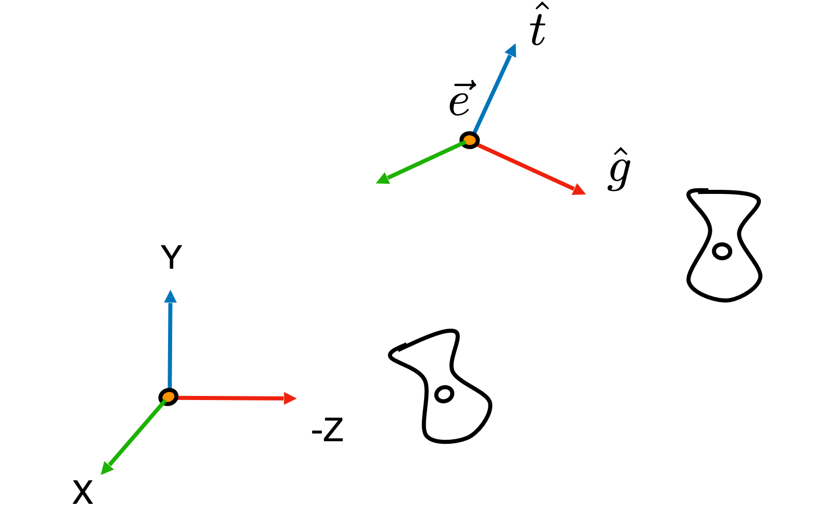
Key observation: If the camera and all objects move together, the “photo” looks the same!
Goal: transform the camera so that it is:
- Located at the origin
- Up direction pointing toward +Y
- Gaze direction pointing toward -Z
Meanwhile transform all objects together.
Deriving the View Transform Matrix
$$ M_{view} = R_{view} \cdot T_{view} $$Step 1: Translation $T_{view}$, move the camera position $\vec{e} = (x_e, y_e, z_e)$ to the origin:
$$ T_{view} = \begin{pmatrix} 1 & 0 & 0 & -x_e \\ 0 & 1 & 0 & -y_e \\ 0 & 0 & 1 & -z_e \\ 0 & 0 & 0 & 1 \end{pmatrix} $$Step 2: Rotation $R_{view}$, align the camera coordinate system with the standard coordinate system:
- Gaze direction $\hat{g}$ → align to the $-Z$ axis
- Up direction $\hat{t}$ → align to the $Y$ axis
- Right direction $\hat{g} \times \hat{t}$ → align to the $X$ axis
Why Is It Easier to Consider the Inverse Rotation?
Difficulty of directly finding $R_{view}$: requires solving complex equations
$$ R_{view} \cdot \hat{g} = -Z, \quad R_{view} \cdot \hat{t} = Y, \quad R_{view} \cdot (\hat{g} \times \hat{t}) = X $$Trick: consider the inverse transform $R_{view}^{-1}$, which does the opposite — maps the standard basis to the camera coordinate system:
$$ R_{view}^{-1} \cdot X = \hat{g} \times \hat{t}, \quad R_{view}^{-1} \cdot Y = \hat{t}, \quad R_{view}^{-1} \cdot Z = -\hat{g} $$The Matrix of the Inverse Rotation $R_{view}^{-1}$
Key observation: each column of the matrix is the transformed basis vector!
| Standard basis | Transform result | Matrix column |
|---|---|---|
| $X = (1,0,0)$ | $\hat{g} \times \hat{t}$ (right) | First column |
| $Y = (0,1,0)$ | $\hat{t}$ (up) | Second column |
| $Z = (0,0,1)$ | $-\hat{g}$ (opposite gaze) | Third column |
Therefore:
$$ R_{view}^{-1} = \begin{pmatrix} | & | & | \\ \hat{g} \times \hat{t} & \hat{t} & -\hat{g} \\ | & | & | \end{pmatrix} = \begin{pmatrix} x_{\hat{g} \times \hat{t}} & x_{\hat{t}} & x_{-\hat{g}} & 0 \\ y_{\hat{g} \times \hat{t}} & y_{\hat{t}} & y_{-\hat{g}} & 0 \\ z_{\hat{g} \times \hat{t}} & z_{\hat{t}} & z_{-\hat{g}} & 0 \\ 0 & 0 & 0 & 1 \end{pmatrix} $$Finding $R_{view}$
The rotation matrix is an orthogonal matrix, satisfying $R^{-1} = R^T$, so:
$$ R_{view} = (R_{view}^{-1})^T $$Transposing turns rows into columns:
$$ R_{view} = \begin{pmatrix} x_{\hat{g} \times \hat{t}} & y_{\hat{g} \times \hat{t}} & z_{\hat{g} \times \hat{t}} & 0 \\ x_{\hat{t}} & y_{\hat{t}} & z_{\hat{t}} & 0 \\ x_{-\hat{g}} & y_{-\hat{g}} & z_{-\hat{g}} & 0 \\ 0 & 0 & 0 & 1 \end{pmatrix} $$Verification
Apply $R_{view}$ to $\hat{g}$ and check whether we get $-Z$:
$$ R_{view} \cdot \hat{g} = \begin{pmatrix} (\hat{g} \times \hat{t}) \cdot \hat{g} \\ \hat{t} \cdot \hat{g} \\ (-\hat{g}) \cdot \hat{g} \\ 0 \end{pmatrix} = \begin{pmatrix} 0 \\ 0 \\ -1 \\ 0 \end{pmatrix} = -Z \quad \checkmark $$Explanation:
- First row: $(\hat{g} \times \hat{t}) \cdot \hat{g} = 0$ (the cross product is perpendicular to the original vector)
- Second row: $\hat{t} \cdot \hat{g} = 0$ (the up direction is perpendicular to the gaze direction)
- Third row: $(-\hat{g}) \cdot \hat{g} = -|\hat{g}|^2 = -1$
10 Projection Transformation
Two Types of Projection
| Projection type | Characteristic | Applications |
|---|---|---|
| Orthographic | Parallel lines stay parallel, no foreshortening | Engineering drawing, CAD |
| Perspective | Parallel lines converge to a point, foreshortening | Games, movies, photorealistic rendering |
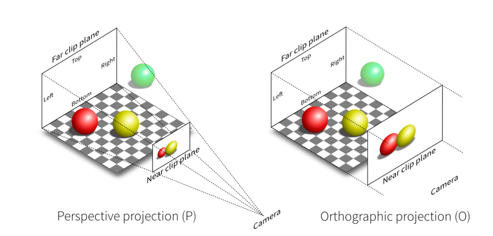
Orthographic Projection
Intuitive understanding:
- The camera is at the origin, looking toward $-Z$, up is $Y$
- Drop the Z coordinate
- Translate and scale the resulting rectangle to $[-1, 1]^2$
General case:
Map the box $[l, r] \times [b, t] \times [f, n]$ to the canonical cube $[-1, 1]^3$.
Where: $l$=left, $r$=right, $b$=bottom, $t$=top, $n$=near, $f$=far.
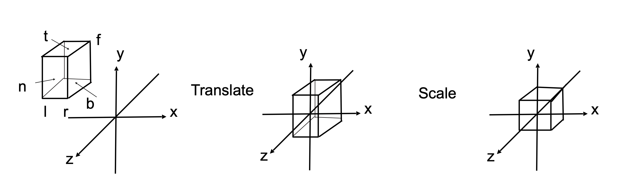
Derivation
Step 1: Translation $T$, move the center of the box to the origin.
The center of the box is $\left(\frac{l+r}{2}, \frac{b+t}{2}, \frac{n+f}{2}\right)$, so the translation is negated:
$$ T = \begin{pmatrix} 1 & 0 & 0 & -\frac{r+l}{2} \\ 0 & 1 & 0 & -\frac{t+b}{2} \\ 0 & 0 & 1 & -\frac{n+f}{2} \\ 0 & 0 & 0 & 1 \end{pmatrix} $$The ranges in each direction after translation become:
| Direction | Original range | Range after translation |
|---|---|---|
| x | $[l, r]$ | $[-\frac{r-l}{2}, \frac{r-l}{2}]$ |
| y | $[b, t]$ | $[-\frac{t-b}{2}, \frac{t-b}{2}]$ |
| z | $[f, n]$ | $[-\frac{n-f}{2}, \frac{n-f}{2}]$ |
Step 2: Scale $S$, scale the box to $[-1, 1]$.
The scale factor in each direction:
| Direction | Range width | Scale factor | Target |
|---|---|---|---|
| x | $r - l$ | $\frac{2}{r-l}$ | $[-1, 1]$ |
| y | $t - b$ | $\frac{2}{t-b}$ | $[-1, 1]$ |
| z | $n - f$ | $\frac{2}{n-f}$ | $[-1, 1]$ |
For example, in the x direction: $\left[-\frac{r-l}{2}\right] \times \frac{2}{r-l} = -1$, $\left[\frac{r-l}{2}\right] \times \frac{2}{r-l} = 1$ ✓
$$ S = \begin{pmatrix} \frac{2}{r-l} & 0 & 0 & 0 \\ 0 & \frac{2}{t-b} & 0 & 0 \\ 0 & 0 & \frac{2}{n-f} & 0 \\ 0 & 0 & 0 & 1 \end{pmatrix} $$Combination: translate first, then scale (matrices are applied right to left).
$$ M_{ortho} = S \cdot T = \begin{pmatrix} \frac{2}{r-l} & 0 & 0 & 0 \\ 0 & \frac{2}{t-b} & 0 & 0 \\ 0 & 0 & \frac{2}{n-f} & 0 \\ 0 & 0 & 0 & 1 \end{pmatrix} \cdot \begin{pmatrix} 1 & 0 & 0 & -\frac{r+l}{2} \\ 0 & 1 & 0 & -\frac{t+b}{2} \\ 0 & 0 & 1 & -\frac{n+f}{2} \\ 0 & 0 & 0 & 1 \end{pmatrix} $$Verification
| Original point | After translation | After scale | Result |
|---|---|---|---|
| $(r, t, n)$ | $(\frac{r-l}{2}, \frac{t-b}{2}, \frac{n-f}{2})$ | $(1, 1, 1)$ | ✓ |
| $(l, b, f)$ | $(-\frac{r-l}{2}, -\frac{t-b}{2}, -\frac{n-f}{2})$ | $(-1, -1, -1)$ | ✓ |
| Center $(\frac{l+r}{2}, \frac{b+t}{2}, \frac{n+f}{2})$ | $(0, 0, 0)$ | $(0, 0, 0)$ | ✓ |
Note: when looking toward $-Z$, the near plane $n > f$ (the near plane has a larger z value), so $n - f > 0$ and the scale factor $\frac{2}{n-f} > 0$.
Perspective Projection
Characteristics:
- Objects farther away appear smaller
- Parallel lines are no longer parallel; they converge to a point (vanishing point)
Important property of homogeneous coordinates:
$(x, y, z, 1)^T$ and $(kx, ky, kz, k)^T$ ($k \neq 0$) represent the same point.
For example: $(x, y, z, 1)$ and $(xz, yz, z^2, z)$ both represent $(x, y, z)$.
Core idea of perspective projection:
- Step 1: “Squish” the frustum into a cuboid
- Near plane unchanged: $n \to n$
- Far plane unchanged: $f \to f$
- Denoted $M_{persp \to ortho}$
- Step 2: apply orthographic projection (we already know how!)
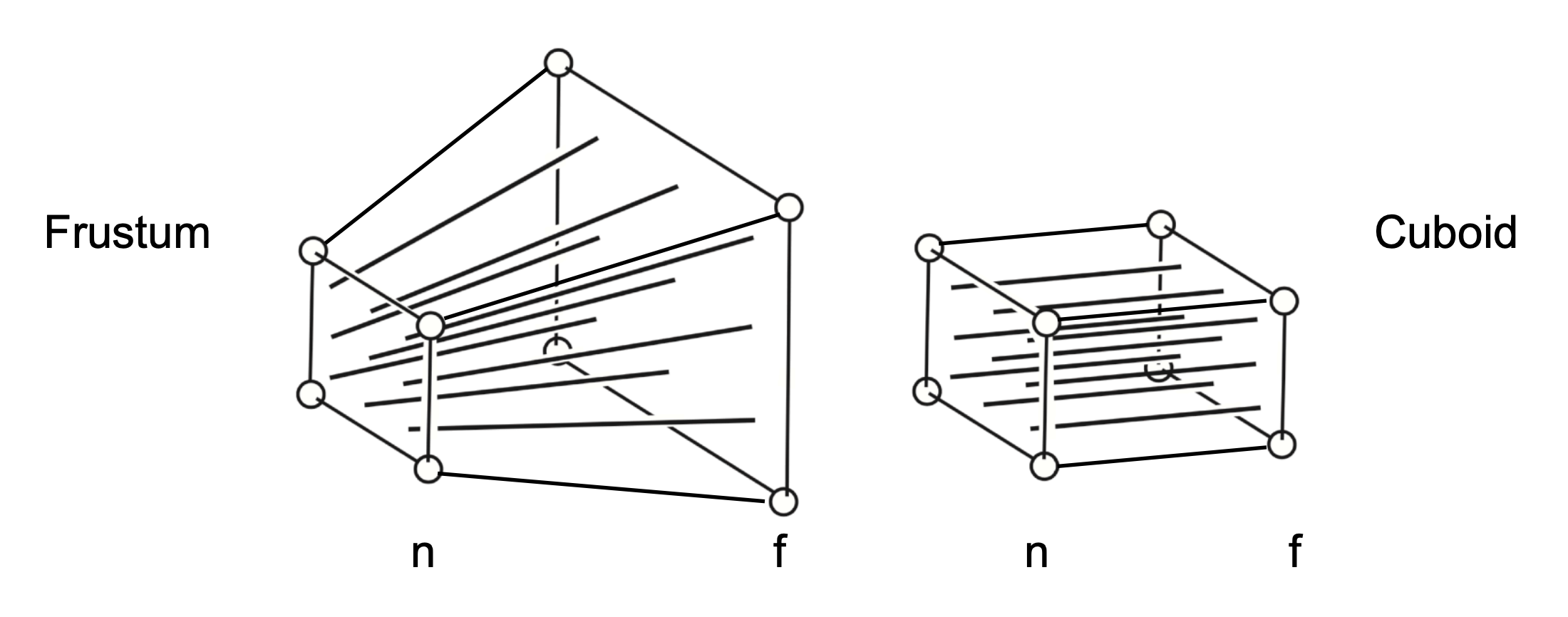
Deriving $M_{persp \to ortho}$:
For a point $(x, y, z)$, after squishing:
- $x' = \frac{n}{z} x$
- $y' = \frac{n}{z} y$
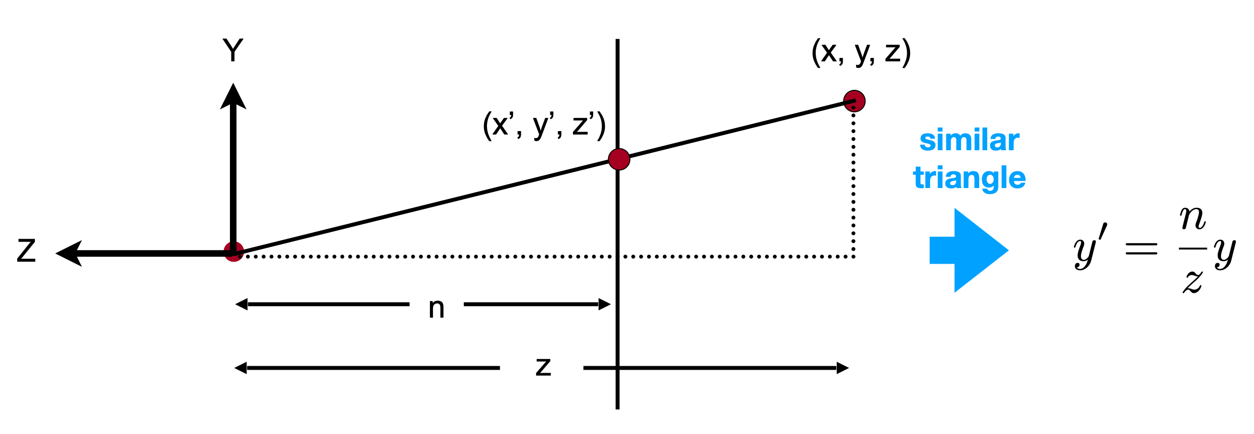
Using homogeneous coordinates:
$$ \begin{pmatrix} x \\ y \\ z \\ 1 \end{pmatrix} \Rightarrow \begin{pmatrix} nx/z \\ ny/z \\ unknown \\ 1 \end{pmatrix} = \begin{pmatrix} nx \\ ny \\ unknown \\ z \end{pmatrix} $$So part of the matrix can be determined:
$$ M_{persp \to ortho} = \begin{pmatrix} n & 0 & 0 & 0 \\ 0 & n & 0 & 0 \\ ? & ? & ? & ? \\ 0 & 0 & 1 & 0 \end{pmatrix} $$Determining the third row:
Use two conditions:
- Points on the near plane are unchanged after the transform ($z = n \to z' = n$), replacing z with n:
The third row:
$$ \begin{pmatrix} 0 & 0 & A & B \end{pmatrix} \begin{pmatrix} x \\ y \\ n \\ 1 \end{pmatrix} = n^2 \quad \Rightarrow \quad A n + B = n^2 $$- Points on the far plane are unchanged after the transform ($z = f \to z' = f$):
Solving the system yields A and B, and the third row is $(0, 0, n+f, -nf)$.
The complete perspective projection matrix:
$$ M_{persp \to ortho} = \begin{pmatrix} n & 0 & 0 & 0 \\ 0 & n & 0 & 0 \\ 0 & 0 & n+f & -nf \\ 0 & 0 & 1 & 0 \end{pmatrix} $$The final perspective projection matrix:
$$ M_{persp} = M_{ortho} \cdot M_{persp \to ortho} $$11 Appendix: Field of View (FOV)
Intuitive Understanding
The Field of View (FOV) describes the angular range the camera can “see”.
Analogous to the human eye: the human field of view is roughly 120° (vertical) × 200° (horizontal). A larger FOV sees a wider range but makes objects appear smaller (like a fisheye lens); a smaller FOV sees a narrower range but makes objects appear larger (like a telescope).
| Type | Description | Typical value |
|---|---|---|
| Vertical FOV (fovY) | Vertical angular range | 45° - 90° |
| Horizontal FOV (fovX) | Horizontal angular range | Determined by fovY and aspect ratio |
Geometric Meaning of FOV
Imagine looking at the near plane from the camera position:
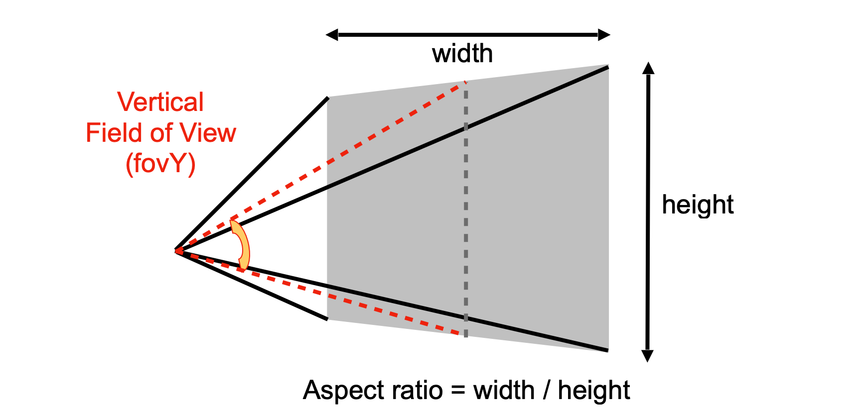
- fovY: the angle between the directions from the camera to the top and bottom of the near plane
- t: half-height of the near plane (from center to top)
- |n|: distance from the camera to the near plane
Deriving the Formula
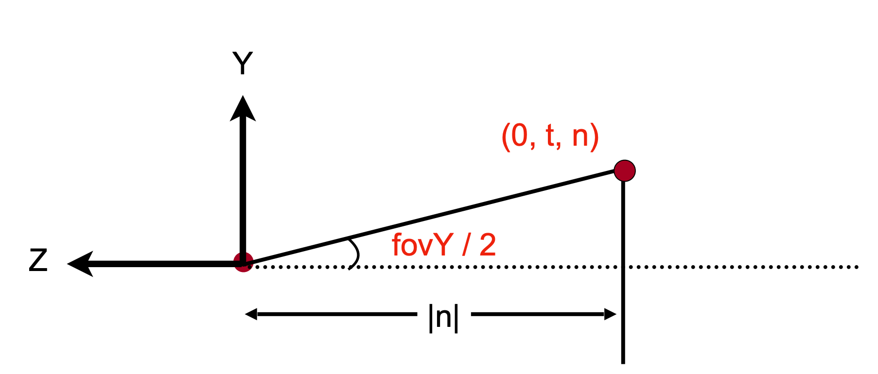
Looking at the near plane from the camera forms a right triangle:
$$ \tan\left(\frac{fovY}{2}\right) = \frac{t}{|n|} $$Where:
- $\frac{fovY}{2}$: the half angle
- $t$: half-height of the near plane (distance from top edge to center)
- $|n|$: near plane distance (camera to near plane, absolute value)
Conversely, if fovY and the near plane distance are known, the near plane range can be found:
$$ t = |n| \cdot \tan\left(\frac{fovY}{2}\right) $$Aspect Ratio
The aspect ratio is defined as:
$$ \text{aspect} = \frac{\text{width}}{\text{height}} = \frac{2r}{2t} = \frac{r}{t} $$where $r$ is the half-width of the near plane.
If the vertical FOV and aspect ratio are known, the horizontal FOV can be found:
$$ \tan\left(\frac{fovX}{2}\right) = \frac{r}{|n|} = \frac{t \cdot \text{aspect}}{|n|} = \text{aspect} \cdot \tan\left(\frac{fovY}{2}\right) $$Practical Application
In games and 3D applications, FOV is an important tunable parameter:
| FOV range | Effect | Applications |
|---|---|---|
| Small FOV (30°-45°) | Narrow view, large objects, “telescope” effect | Sniper scopes, cinematic lenses |
| Medium FOV (60°-90°) | Moderate view, more realistic | Default for most games |
| Large FOV (90°-120°) | Wide view, small objects, “fisheye” effect | VR, racing games |
Example: if fovY = 60° and the near plane distance |n| = 1, then:
$$ t = 1 \cdot \tan(30°) = \frac{1}{\sqrt{3}} \approx 0.577 $$If aspect = 16:9, then:
$$ r = t \cdot \text{aspect} = 0.577 \times \frac{16}{9} \approx 1.026 $$This determines the near plane range $[-r, r] \times [-t, t] = [-1.026, 1.026] \times [-0.577, 0.577]$.
12 Self-Check
Why is translation not a linear transform? How do homogeneous coordinates solve this?
Why is the w coordinate 1 for points but 0 for vectors in matrix multiplication?
Why is rotation about an arbitrary point decomposed into “translate → rotate → translate”?
Why does the view transform first find the inverse rotation $R_{view}^{-1}$, then transpose to obtain $R_{view}$?
How is the third row of the perspective projection matrix $M_{persp \to ortho}$ solved using the near and far plane conditions?
What is the relationship between FOV, the near plane range, and the aspect ratio?
This is note 3 of the GAMES101 - Modern Computer Graphics learning series.