Instructor: Lingqi Yan | UCSB Bilibili: https://www.bilibili.com/video/BV1X7411F744 Lectures covered: Lecture 7 (Illumination, Shading and Graphics Pipeline), Lecture 8 (Shading, Pipeline and Texture Mapping), Lecture 9 (Texture Mapping cont.)
Note: In the official condensed slides, texture applications (environment maps, bump/normal/displacement maps, 3D textures) appear in Lecture 10 and shadow mapping in Lecture 12; following the full Bilibili course structure, they are grouped under the shading topic here.
Shading is the process of applying material properties to objects, which determines their color and appearance under different lighting conditions. This post covers the depth buffer (visibility/occlusion), the Blinn-Phong reflectance model, shading frequencies, the graphics pipeline, texture mapping and related techniques.
1 Depth Buffer (Z-Buffer)
The Problem
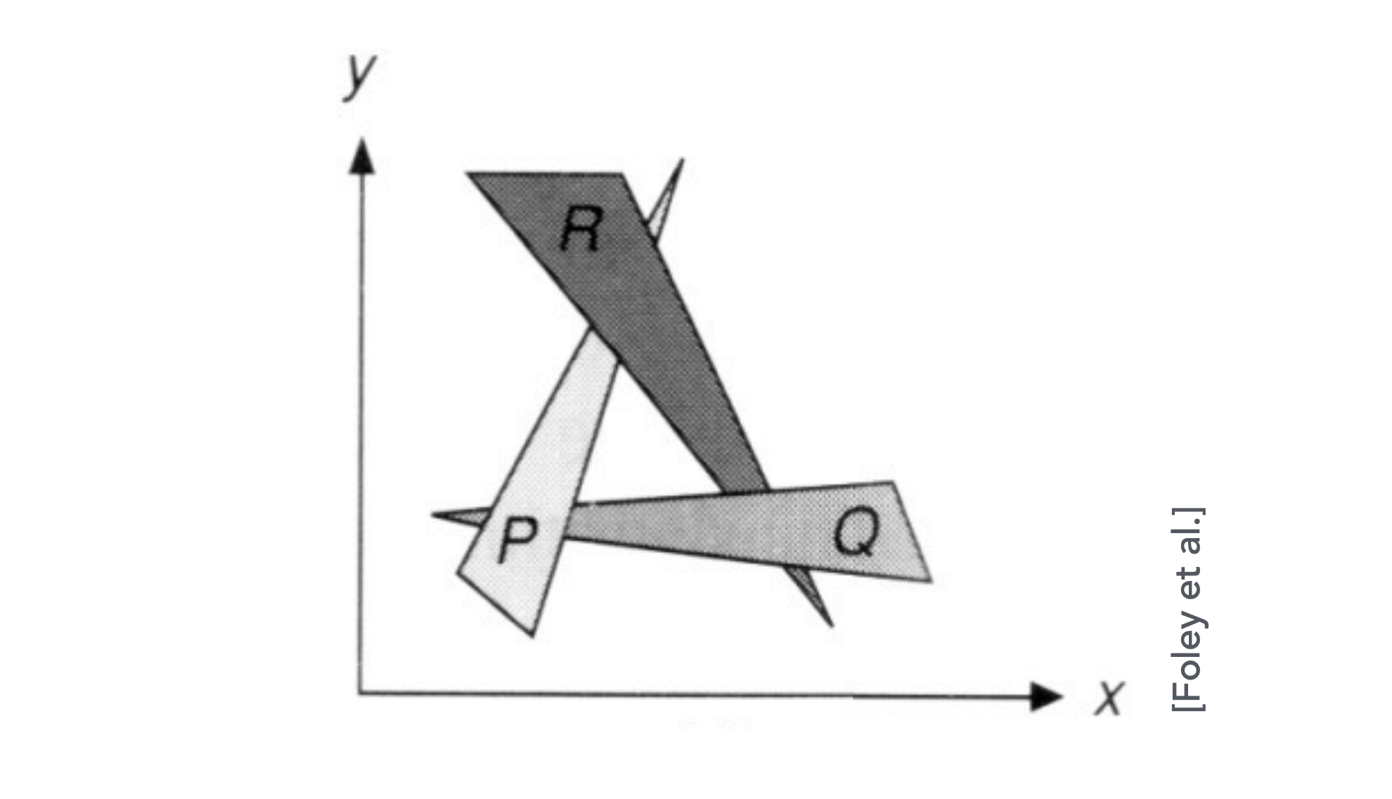
Multiple triangles may cover the same pixel — how do we decide which triangle is in front?
Painter’s Algorithm
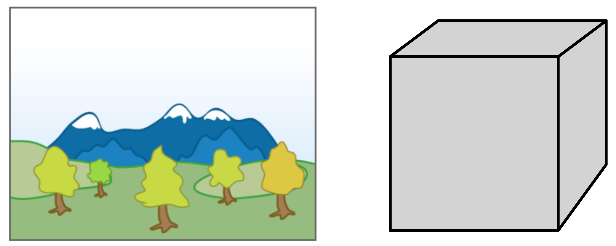
Idea: draw far objects first, then near ones (near objects overwrite far ones in the framebuffer during drawing).
Problems:
- Requires depth-sorting all triangles ($O(n \log n)$, n = number of triangles), which is expensive
- Cyclic occlusion may occur, making the depth order impossible to determine (unresolvable depth order)
Z-Buffer Algorithm
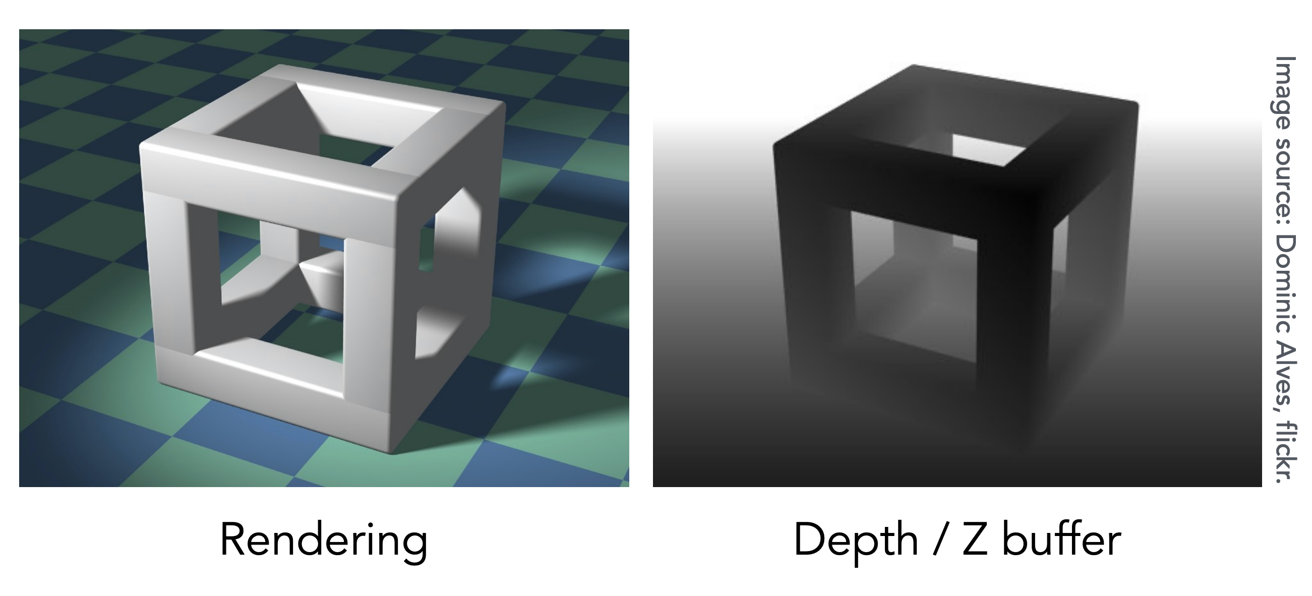
Core idea: store the current minimum depth $z$ for each sample (pixel) and compare depths during rendering (this is the visibility algorithm that ultimately won).
Simplifying assumption (emphasized in the slides): $z$ is always positive, smaller z → closer, larger z → further.
Data structures:
- Framebuffer: stores the color of each pixel
- Depth Buffer (Z-Buffer): stores the depth of each pixel
Algorithm flow:
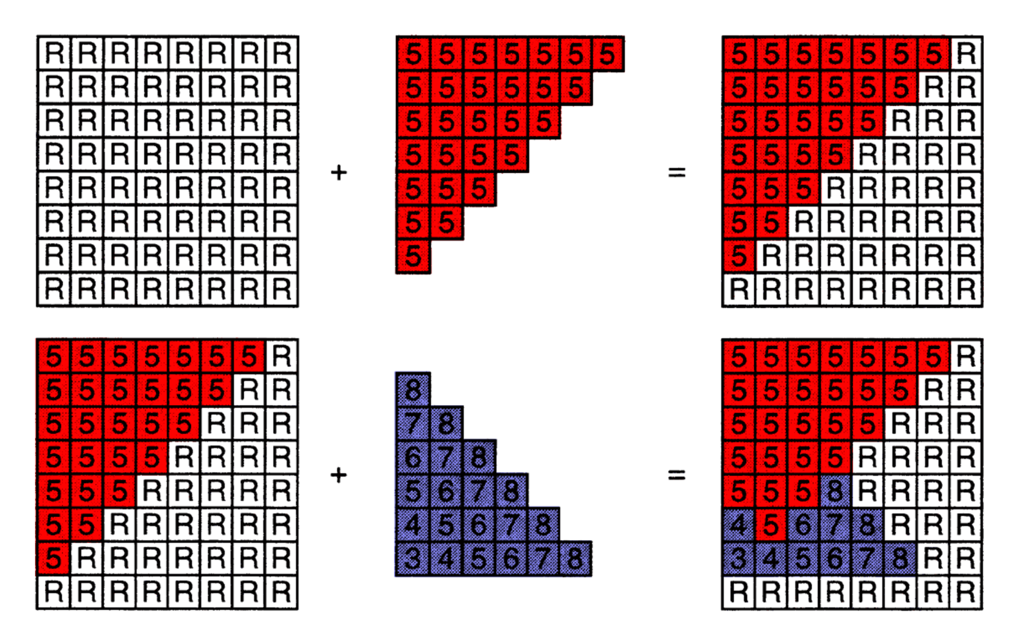
- Initialize: set every depth buffer entry to infinity (farthest), set the framebuffer to the background color
- Iterate over triangles: process each triangle in the scene one by one
- Rasterize: for each sample $(x, y, z)$ of the current triangle, compute its screen-space position and depth
- Depth test: compare the sample’s depth $z$ with the depth already stored for that pixel
- Update condition: only when $z$ is smaller (closer to the camera), replace the pixel’s color and depth
- Repeat: run the above for all triangles; the framebuffer finally holds the visible image
// Initialization: fill depth buffer with infinity
for each pixel (x, y):
    zbuffer[x][y] = ∞  // initialize to maximum depth
    framebuffer[x][y] = background_color

// Rendering
for each triangle T:
    for each sample (x, y, z) in T:
        if z < zbuffer[x, y]:        // closest sample so far
            framebuffer[x, y] = rgb  // update color
            zbuffer[x, y] = z        // update depth
        else:
            ;                        // do nothing, sample is occluded
Key properties:
- Time complexity: $O(n)$, n = number of triangles (assuming constant coverage per triangle)
- No sorting of triangles required
- Each triangle is processed independently, regardless of drawing order
- The most important visibility algorithm — implemented in hardware on every GPU
Caveats:
- Depth values are usually nonlinear (after perspective projection)
- Finite depth precision can cause Z-fighting
2 Shading Basics
In Merriam-Webster, shading is defined as “degreed darkness or coloration of a picture or diagram by means of parallel lines or masses of color.”
In computer graphics, shading is the process of applying materials to objects.
Shading considers three key ingredients:
| Ingredient | Description |
|---|---|
| Material properties | Surface color, shininess, reflectance, etc. |
| Lighting | Light source intensity, direction, color |
| View direction | The direction from which the camera looks at the object |
3 Blinn-Phong Reflectance Model
Model Overview
The Blinn-Phong reflectance model is a simple but practical empirical lighting model that splits illumination into three components:
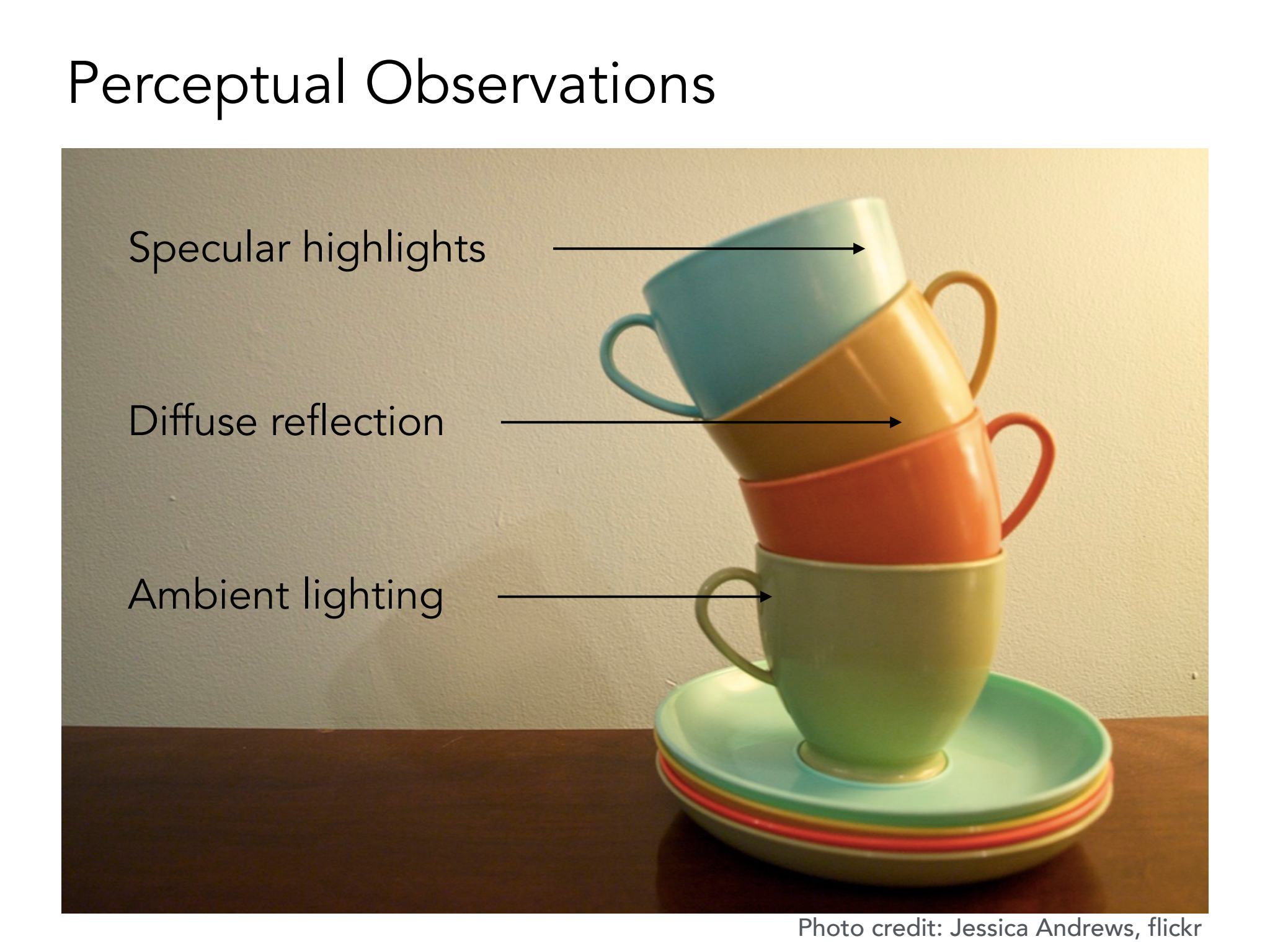
| Component | Name | Characteristics |
|---|---|---|
| Specular highlights | Specular | Mirror-like reflection, view-dependent |
| Diffuse reflection | Diffuse | Light scattered evenly, view-independent |
| Ambient lighting | Ambient | Constant term approximating indirect light |
Shading Is Local
Shading computes the light reflected toward the camera at a specific shading point. The inputs are:
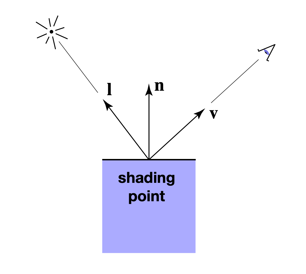
| Input | Symbol | Description |
|---|---|---|
| View direction | $\vec{v}$ | Unit vector from the shading point toward the camera |
| Surface normal | $\vec{n}$ | Unit vector perpendicular to the surface at the shading point |
| Light direction | $\vec{l}$ | Unit vector from the shading point toward the light (one per light) |
| Surface params | — | Color, shininess, etc. |
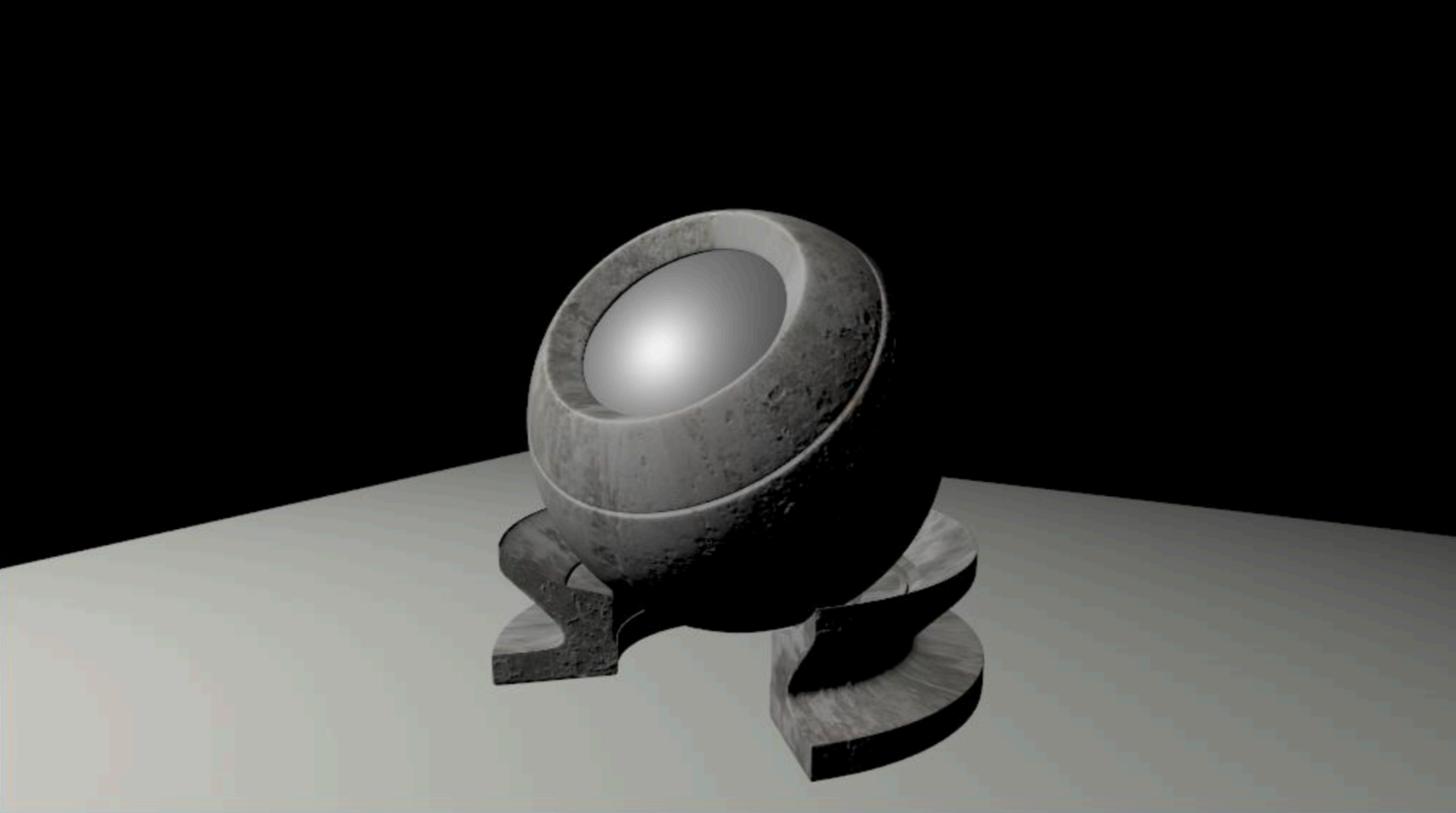
Key property: shading is local — it only uses information at the point itself and cannot produce shadows (shading ≠ shadow), because it has no knowledge of other objects in the scene.
Diffuse Reflection
Diffuse reflection is the phenomenon where light hitting a rough surface is scattered evenly in all directions.
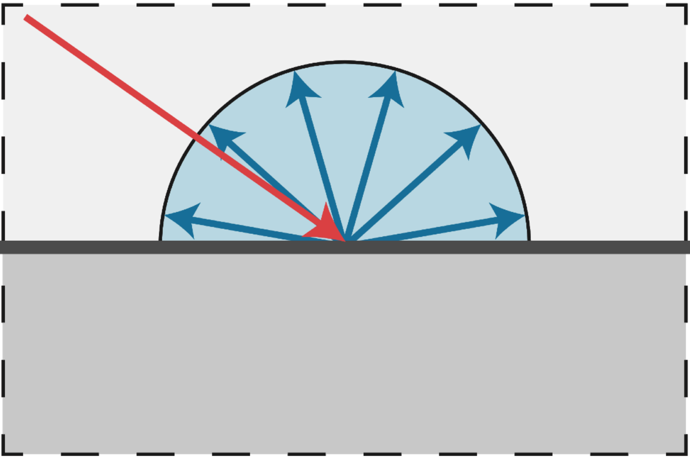
Basic Principles
- Isotropic scattering: incident light is dispersed over the hemisphere of directions
- View-independent: brightness looks essentially the same from any viewpoint (Lambert’s cosine law)
- No mirror image: unlike specular reflection, no clear image is formed
The core property of diffuse reflection: light is scattered evenly in all directions, so surface color is independent of the view direction.
Lambert’s Cosine Law
The light energy reaching a surface depends on the angle between the light direction and the normal.
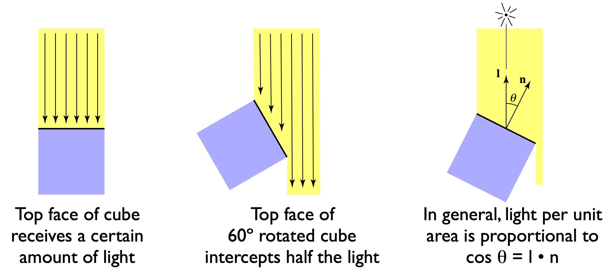
- When the cube’s top face is perpendicular to the light, it receives all the illumination
- After rotating 60°, the same area receives only half of the light
- In general, light energy per unit area is proportional to $\cos\theta = \vec{l} \cdot \vec{n}$
where $\theta$ is the angle between the light direction $\vec{l}$ and the surface normal $\vec{n}$.
Light Attenuation
Once emitted from a point light, energy attenuates with distance.
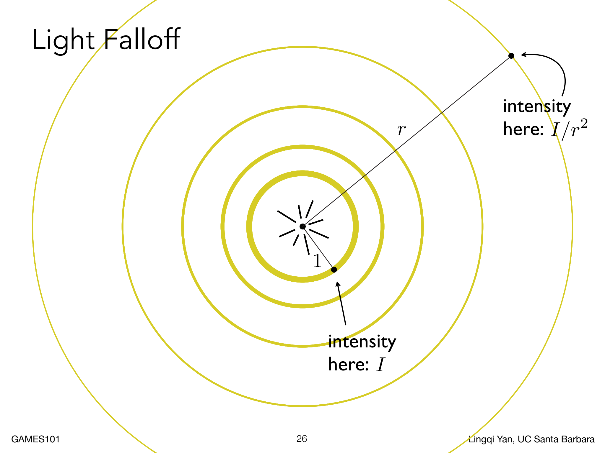
At distance $r$, the light intensity is $\frac{I}{r^2}$ (a point light radiates in all directions, spreading energy over a larger sphere):
$$ I(r) = \frac{I}{r^2} $$where $I$ is the light intensity at unit distance.
Diffuse Formula
Combining Lambert’s cosine law and attenuation, the diffuse shading term is:
$$ L_d = k_d \cdot \frac{I}{r^2} \cdot \max(0, \vec{n} \cdot \vec{l}) $$| Symbol | Meaning |
|---|---|
| $L_d$ | Diffuse light (the color ultimately seen) |
| $k_d$ | Diffuse coefficient (diffuse reflectance, representing surface color) |
| $I$ | Light intensity |
| $r$ | Distance from shading point to light |
| $\vec{n} \cdot \vec{l}$ | Dot product of normal and light direction ($\cos\theta$) |
| $\max(0, \cdot)$ | Clamps negatives (back-facing surfaces receive no light) |
Effect of $k_d$: larger $k_d$ → brighter surface; $k_d = 0$ means no diffuse reflection at all.
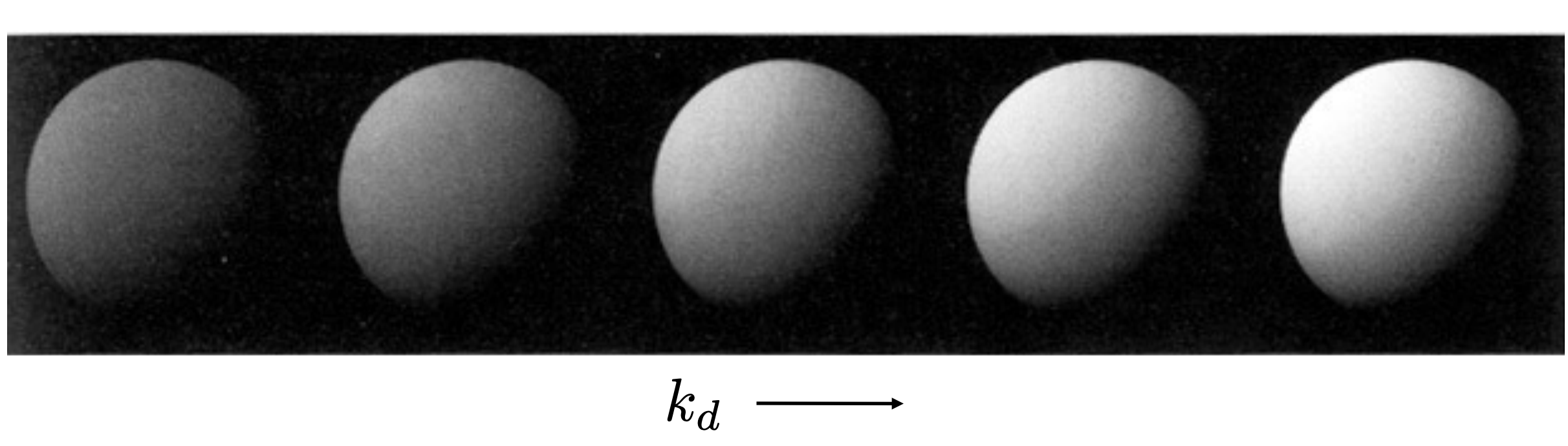
Note: diffuse reflection is independent of the view direction $\vec{v}$ — it looks the same from every angle.
Specular Reflection
Basic Principles
Specular intensity depends on the view direction: it looks brightest near the perfect mirror-reflection direction.
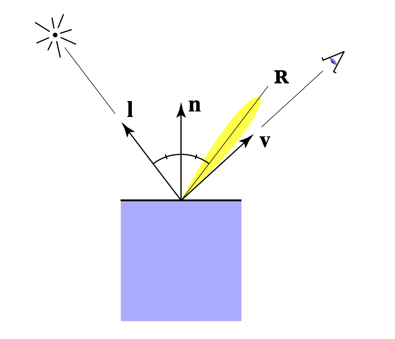
Half Vector
The Blinn-Phong model introduces the half vector to simplify computation:
$$ \vec{h} = \text{bisector}(\vec{v}, \vec{l}) = \frac{\vec{v} + \vec{l}}{\|\vec{v} + \vec{l}\|} $$When $\vec{h}$ exactly equals the surface normal $\vec{n}$, the light and view directions are symmetric about the normal.
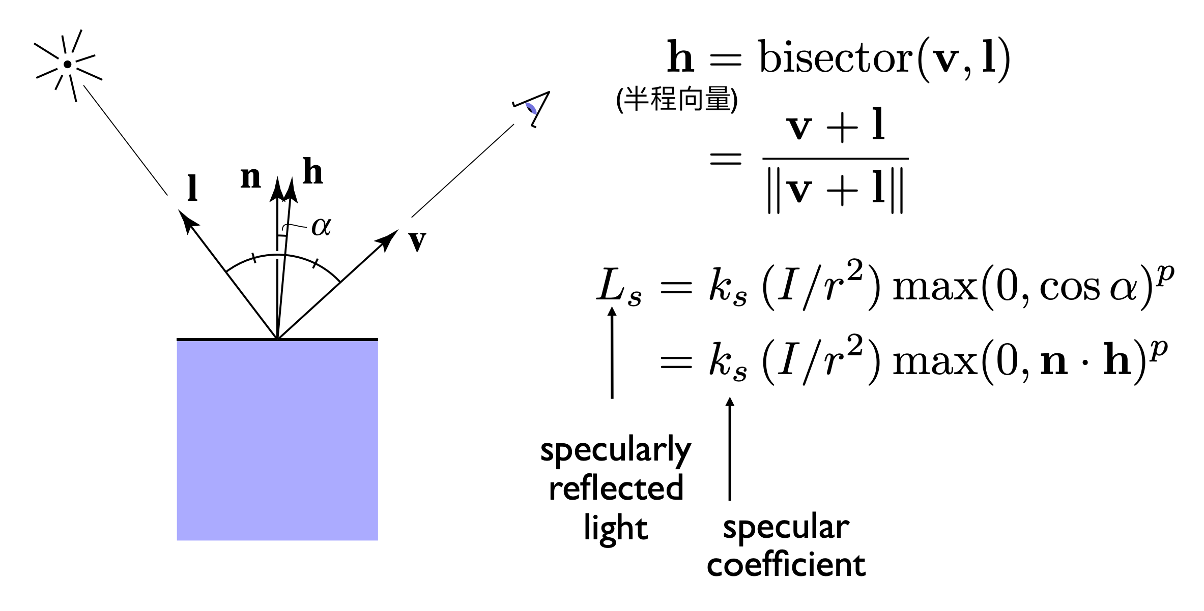
Core idea: $\vec{v}$ being close to the mirror-reflection direction is equivalent to $\vec{h}$ being close to $\vec{n}$. The dot product of unit vectors measures this closeness: $\vec{n} \cdot \vec{h} = \cos\alpha$.
Why the half vector instead of computing the reflection direction directly? Because it only needs a vector addition and normalization, while computing the reflection direction costs more operations.
Role of the Exponent p
Using $\cos\alpha$ directly as specular intensity gives highlights that are far too broad. Introducing the exponent $p$ shrinks the highlight (narrows the reflection lobe):
$$ \max(0, \cos\alpha)^p $$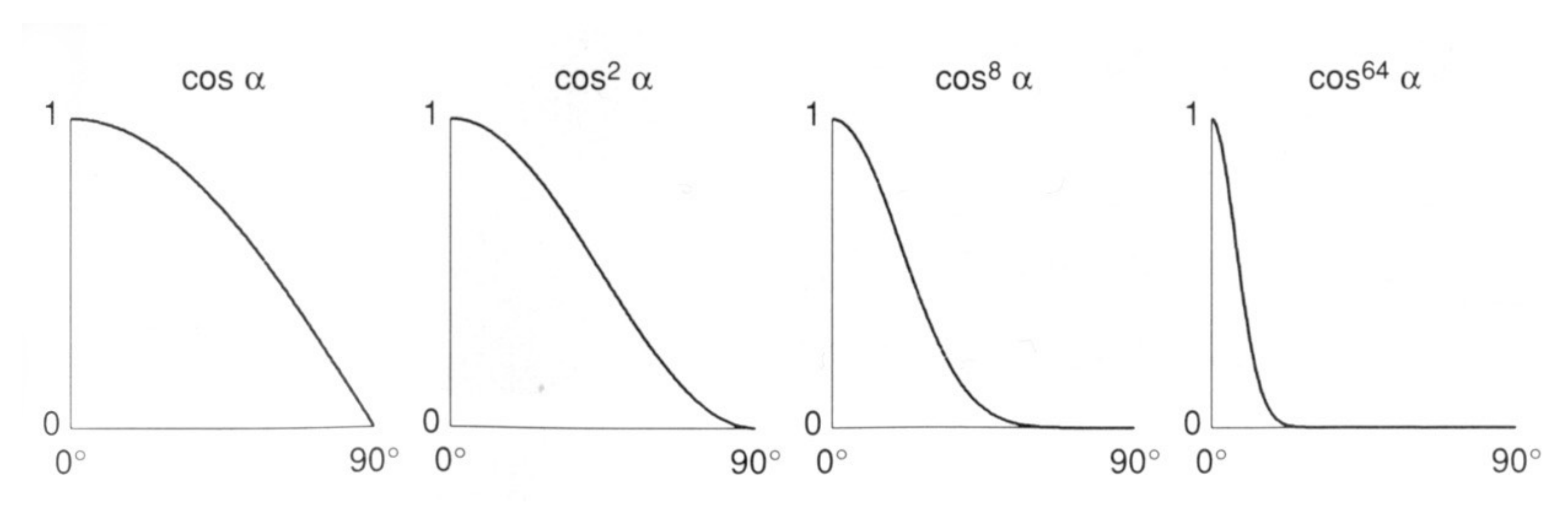
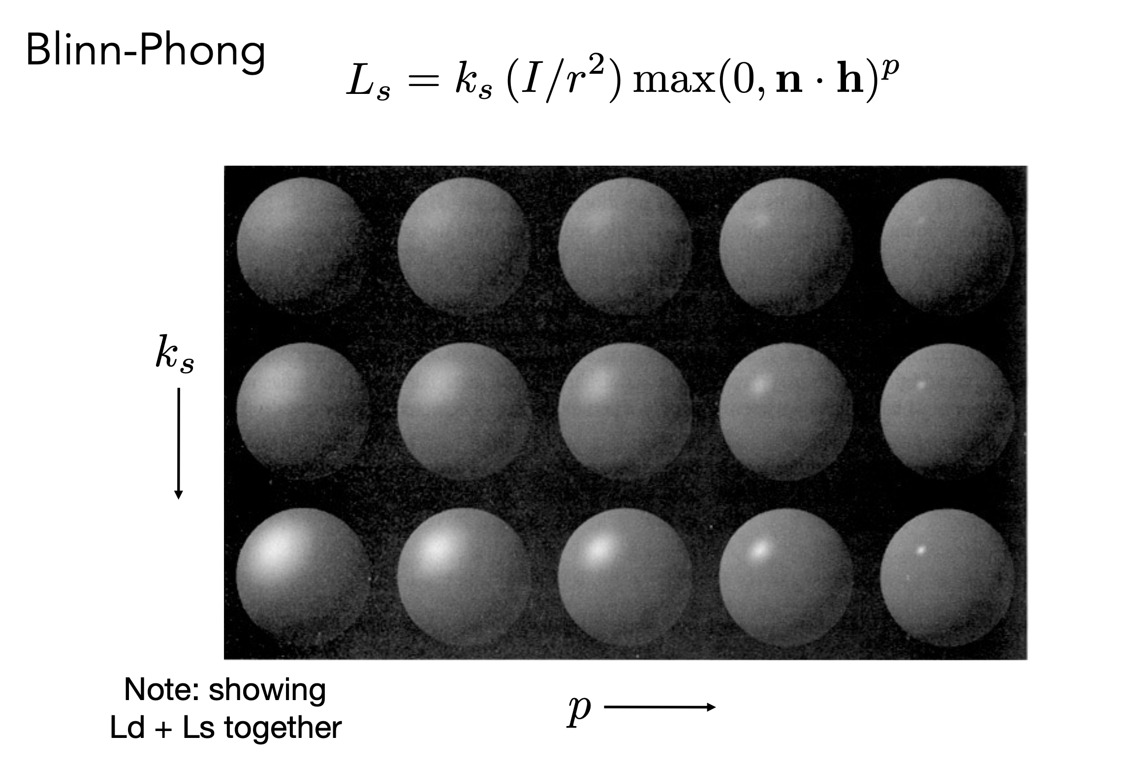
| Exponent $p$ | Effect |
|---|---|
| $p = 1$ | Very broad highlight, unnatural |
| $p = 64$ | Reasonable highlight size |
| $p = 128$ | Small highlight, close to a real mirror |
| $p \to \infty$ | Approaches perfect mirror reflection |
Increasing $p$ narrows the reflection lobe, concentrating the highlight.
The slides also show a comparison sweep with $k_s$ from 0 to 1 and gradually increasing $p$: larger $k_s$ → brighter highlight; larger $p$ → smaller highlight, closer to mirror-like. Note the comparison images show the combined $L_d + L_s$ result, not the specular term alone.
Specular Formula
$$ L_s = k_s \cdot \frac{I}{r^2} \cdot \max(0, \vec{n} \cdot \vec{h})^p $$| Symbol | Meaning |
|---|---|
| $L_s$ | Specular light |
| $k_s$ | Specular coefficient (mirror reflectance) |
| $\vec{h}$ | Half vector |
| $p$ | Specular exponent (controls highlight size) |
Ambient Light
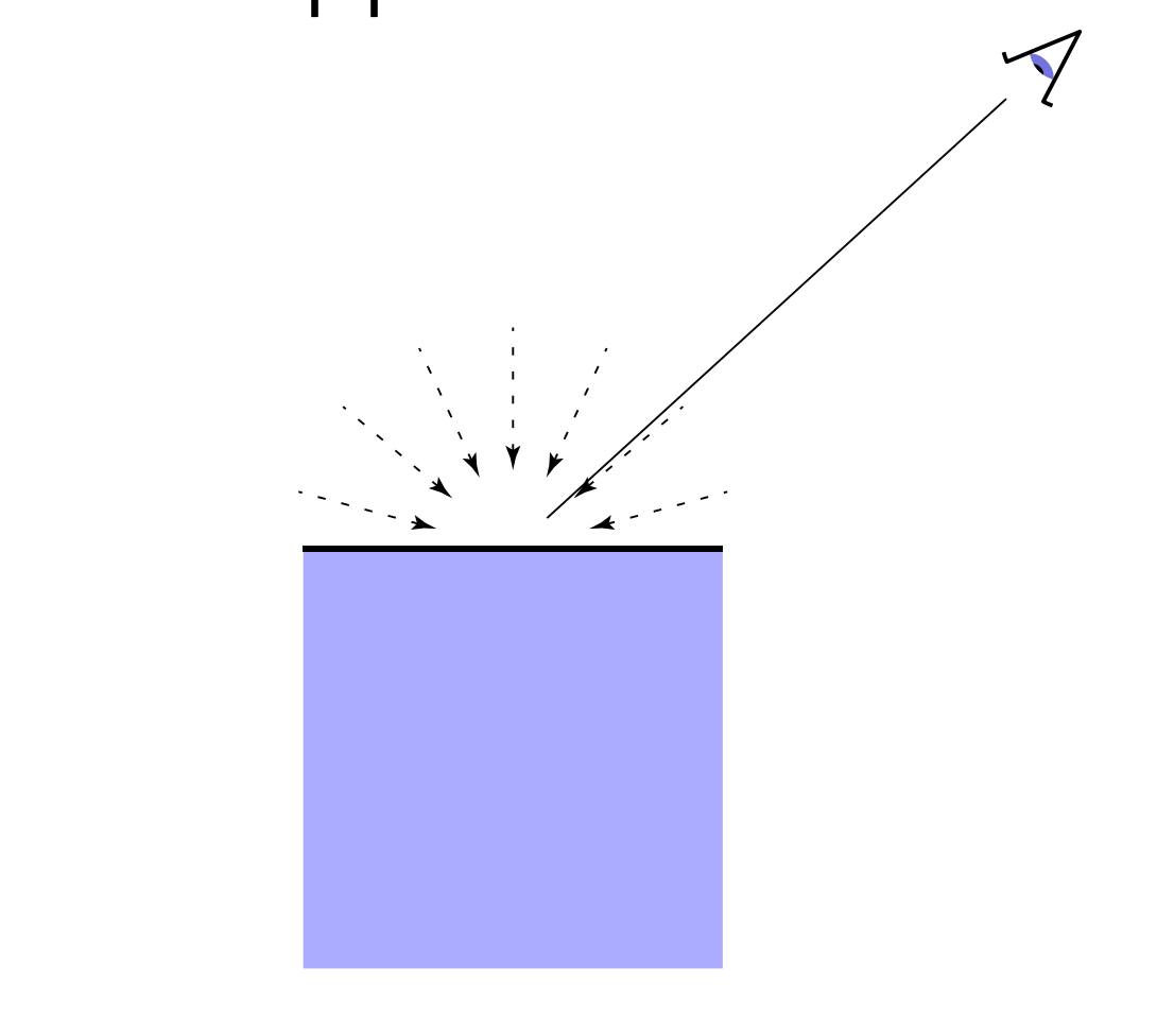
Ambient light is shading that depends on nothing: add a constant color to approximate the ignored indirect illumination and fill in the black shadowed regions.
| Symbol | Meaning |
|---|---|
| $L_a$ | Ambient light (reflected ambient) |
| $k_a$ | Ambient coefficient |
| $I_a$ | Ambient light intensity |
Characteristics:
- A constant color approximating neglected indirect lighting
- Fills shadowed regions to avoid pure black
- This is an approximation / fake — not real global illumination
Full Blinn-Phong Model
Summing the three components gives the complete Blinn-Phong reflectance model:
$$ L = L_a + L_d + L_s = k_a I_a + k_d \frac{I}{r^2} \max(0, \vec{n} \cdot \vec{l}) + k_s \frac{I}{r^2} \max(0, \vec{n} \cdot \vec{h})^p $$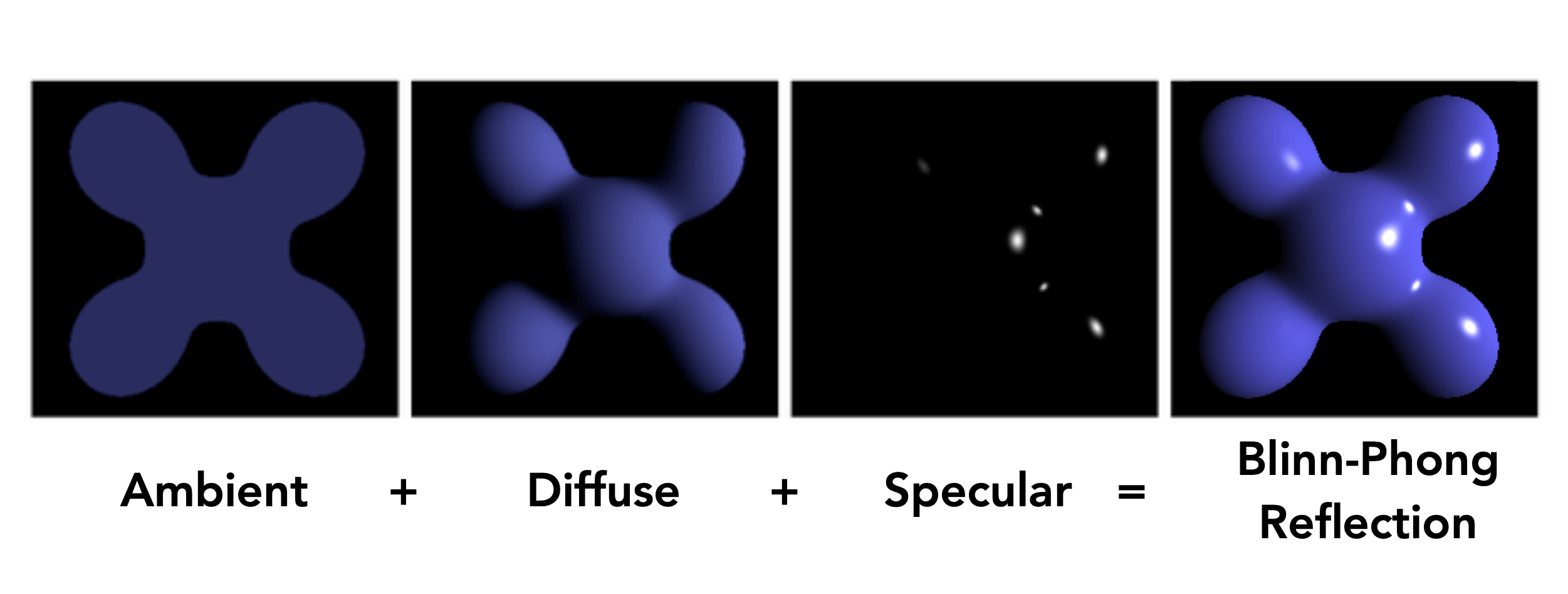
4 Shading Frequencies
Three Shading Frequencies
What shading differences do you see between the three spheres below?
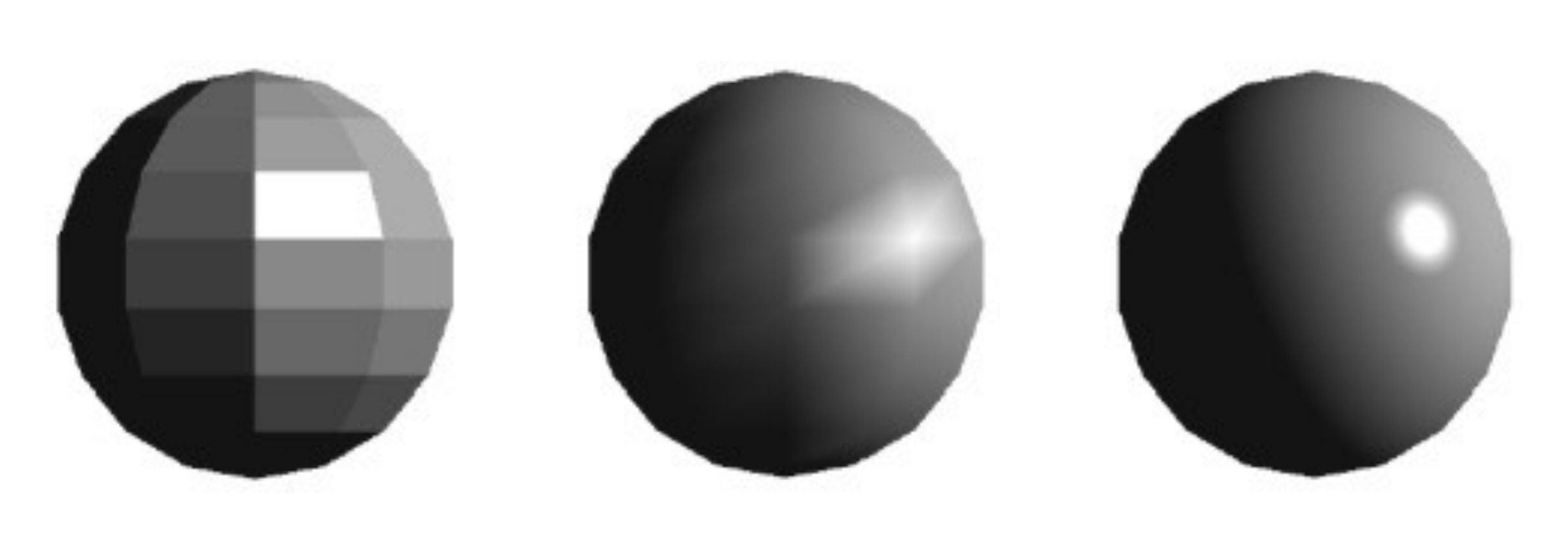
The same geometry shaded at different frequencies produces dramatically different results. From left to right: shading applied to faces, vertices, and pixels.
Flat Shading
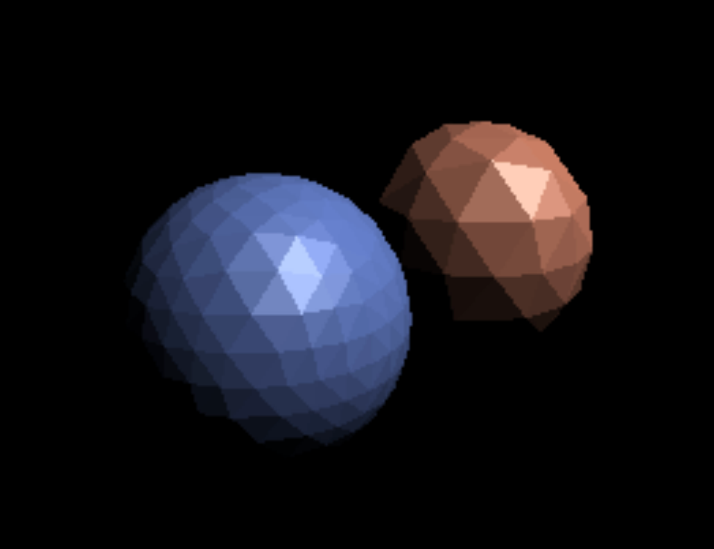
- Shaded on: each triangle (face)
- Method: one normal per face; the whole face gets a single color
- Property: faces stay flat — suitable for faceted objects
- Drawback: bad for smooth surfaces; triangle edges are clearly visible
Gouraud Shading (Vertex Shading)
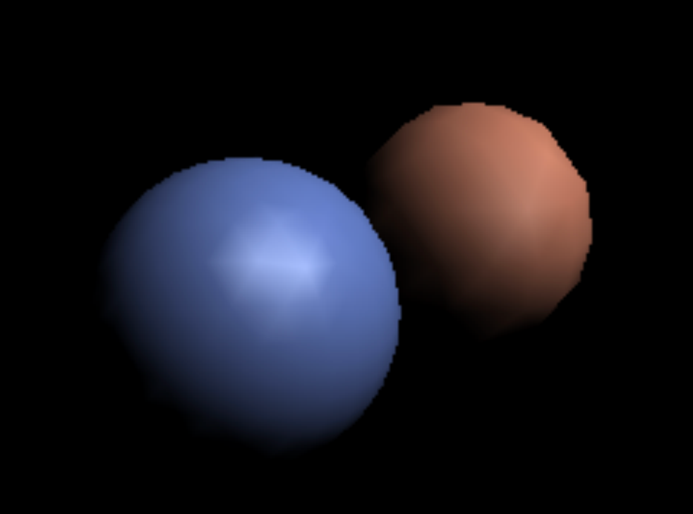
- Shaded on: each vertex
- Method: compute color at each vertex, then interpolate across the triangle
- Property: colors vary smoothly within triangles
- Problem: highlights may be lost if a highlight falls inside a triangle rather than at a vertex
Phong Shading (Pixel Shading)
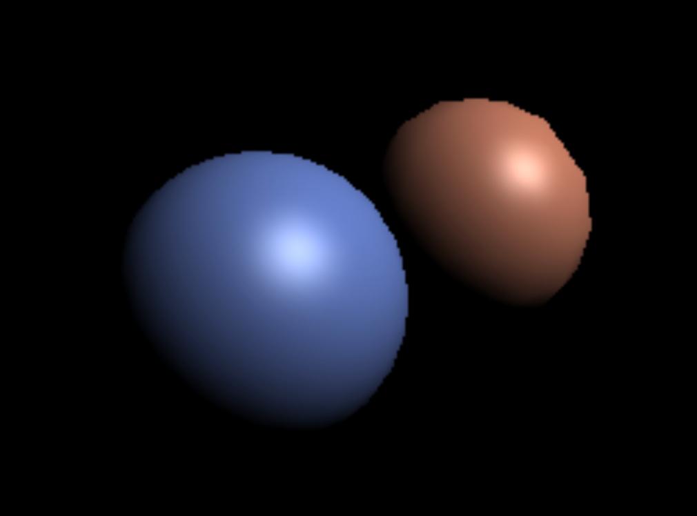
- Shaded on: each pixel
- Method: interpolate the normal per pixel, then evaluate the full shading model at every pixel
- Property: the smoothest result
- Note: Phong Shading (a shading frequency) ≠ Blinn-Phong Reflectance Model (a lighting model) — they are different concepts
Comparison of the Three Frequencies
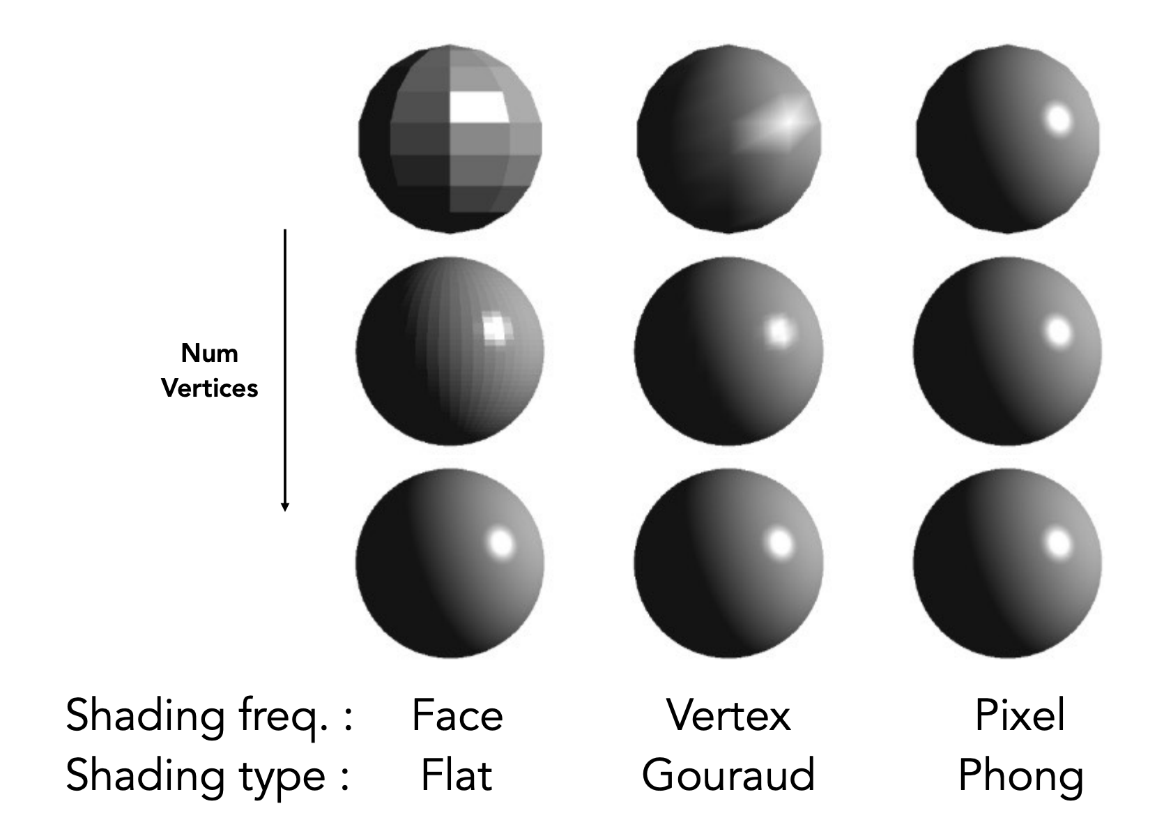
| Frequency | Shaded on | Normal source | Quality | Cost |
|---|---|---|---|---|
| Flat | Face | Face normal | Faceted | Lowest |
| Gouraud | Vertex | Vertex normal | Fairly smooth | Medium |
| Phong | Pixel | Interpolated normal | Smoothest | Highest |
When to choose which? If the geometry is dense enough (small enough triangles), even flat shading can look good. The choice of shading frequency is a balance between geometric accuracy and performance.
Computing Vertex Normals
The best source of vertex normals is the underlying geometry itself (e.g. a sphere’s vertex normals point from the center to each vertex).
When unavailable, infer them from adjacent triangle faces:
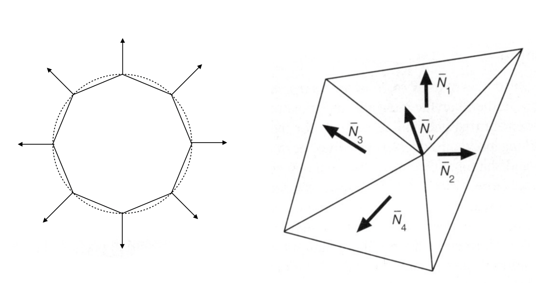
That is, average (or weight-average) the normals of all adjacent faces around the vertex, then normalize.
Computing Pixel Normals
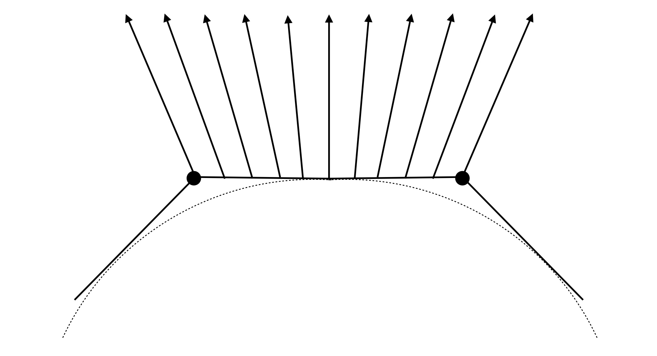
Obtain each pixel’s normal by barycentric interpolation (Section 7) of the vertex normals.
Important reminder: always renormalize the interpolated normal.
5 Graphics Pipeline
Full Flow
The graphics rendering pipeline describes the whole process from 3D vertex input to 2D image output:
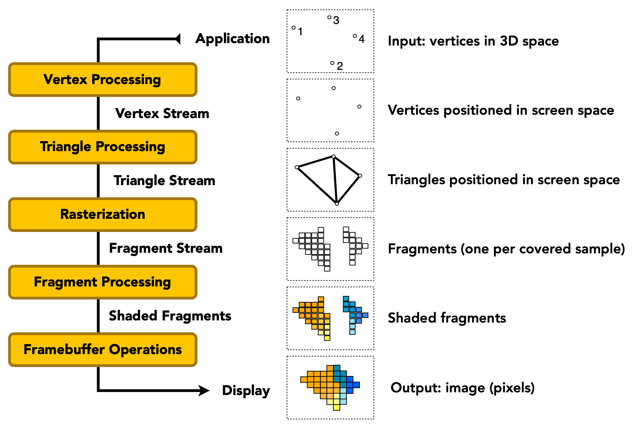
| Stage | Input | Processing | Output |
|---|---|---|---|
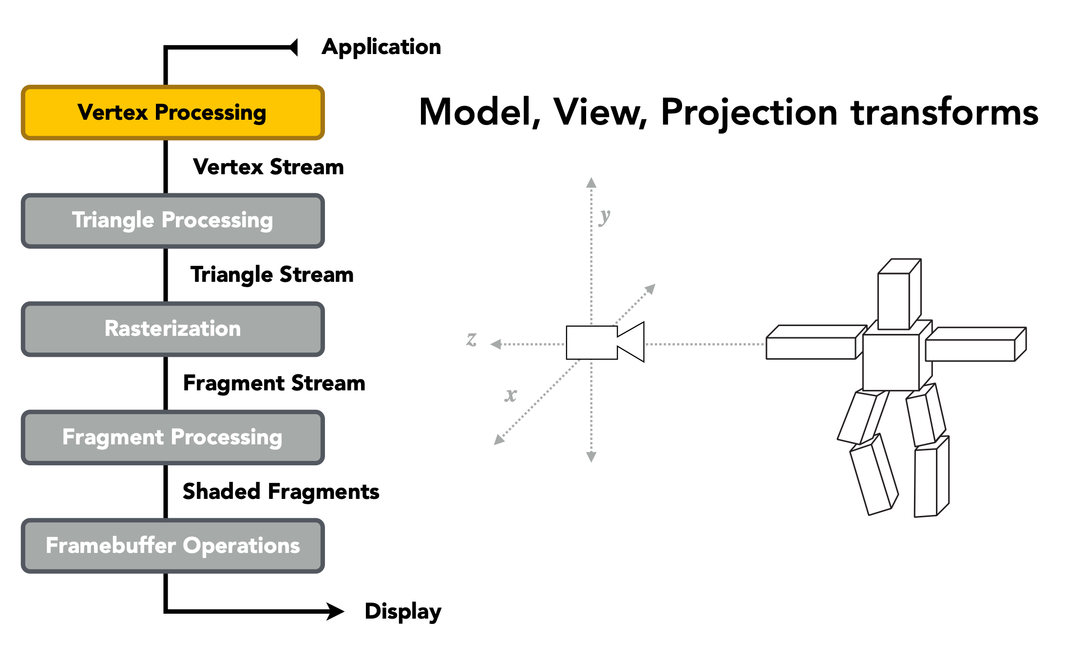
| Vertex Processing | Vertices in 3D space | MVP transforms, vertex shading | Vertices in screen space |
| Triangle Processing | Vertex stream | Assemble triangles | Triangle stream |
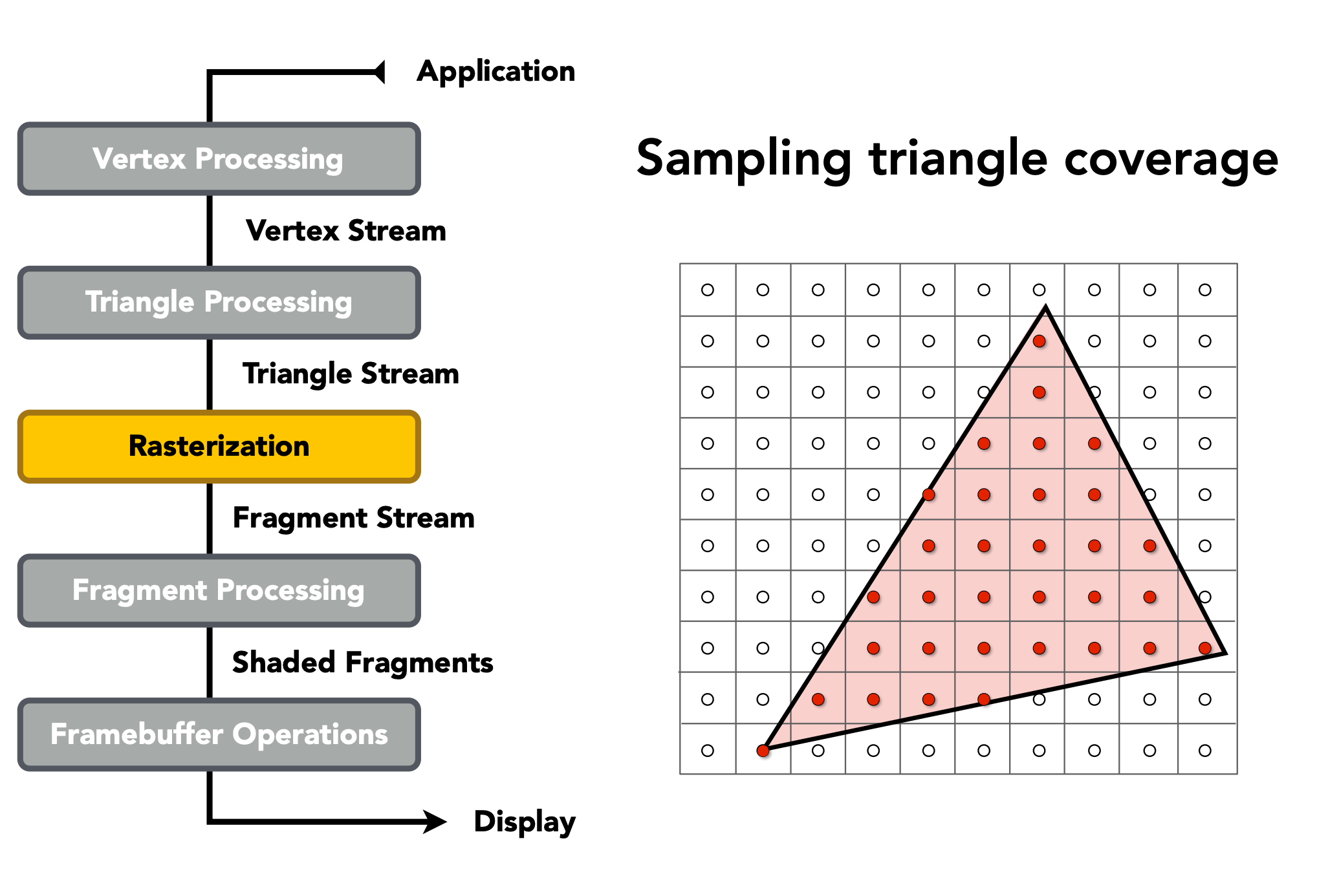
| Rasterization | Triangles | Sample triangle coverage | Fragment stream (one fragment per covered sample) |
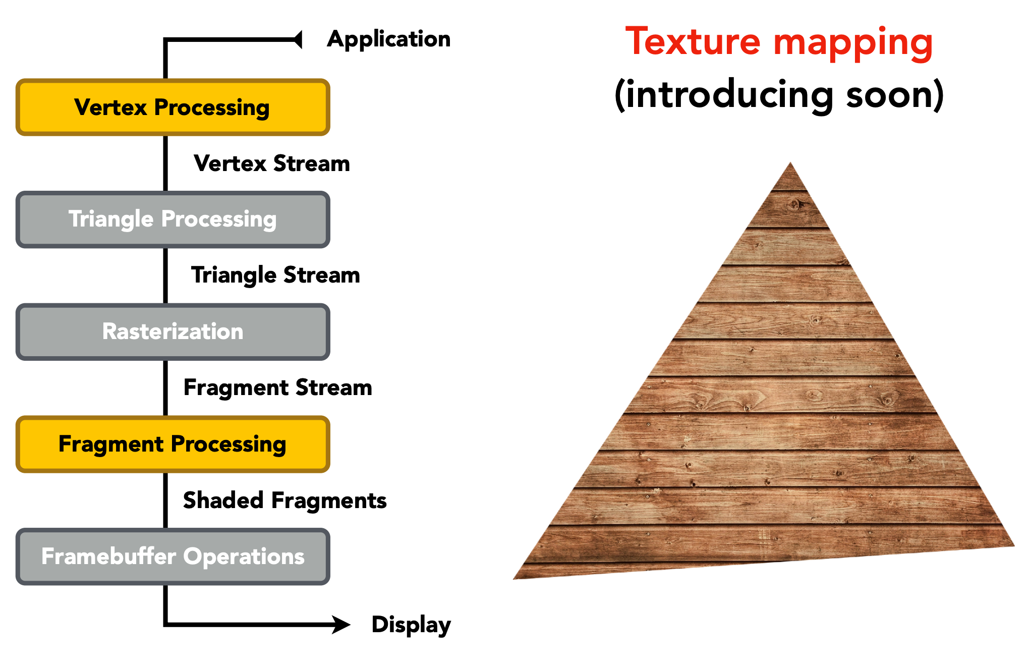
| Fragment Processing | Fragments | Z-buffer depth test, shading (Blinn-Phong), texture mapping | Shaded fragments |
| Framebuffer Operations | Shaded fragments | Write to framebuffer | Final image |
Concrete examples of what each pipeline stage actually processes:


Shader Programs
Modern graphics APIs (e.g. OpenGL) let programmers customize the vertex and fragment processing stages via shaders.
A shader describes the operation on a single vertex (or single fragment), executed for every vertex or pixel fragment.
Example GLSL fragment shader (runs once per fragment):
uniform sampler2D myTexture;   // program parameters: texture
uniform vec3 lightDir;         // program parameters: light direction
varying vec2 uv;               // per-fragment values (interpolated by rasterizer)
varying vec3 norm;             // per-fragment values (interpolated) vertex normal

void diffuseShader()
{
    vec3 kd;  // coefficient
    kd = texture2d(myTexture, uv);           // material color from texture
    kd *= clamp(dot(-lightDir, norm), 0.0, 1.0); // Lambertian shading
    gl_FragColor = vec4(kd, 1.0);            // output fragment color
}
Notes:
uniform: program-level parameters shared by all fragments, global variablesvarying: per-fragment values interpolated from vertices by the rasterizer- The output color is written to
gl_FragColor - The shader runs once per fragment, producing the surface color at that fragment’s screen sample location
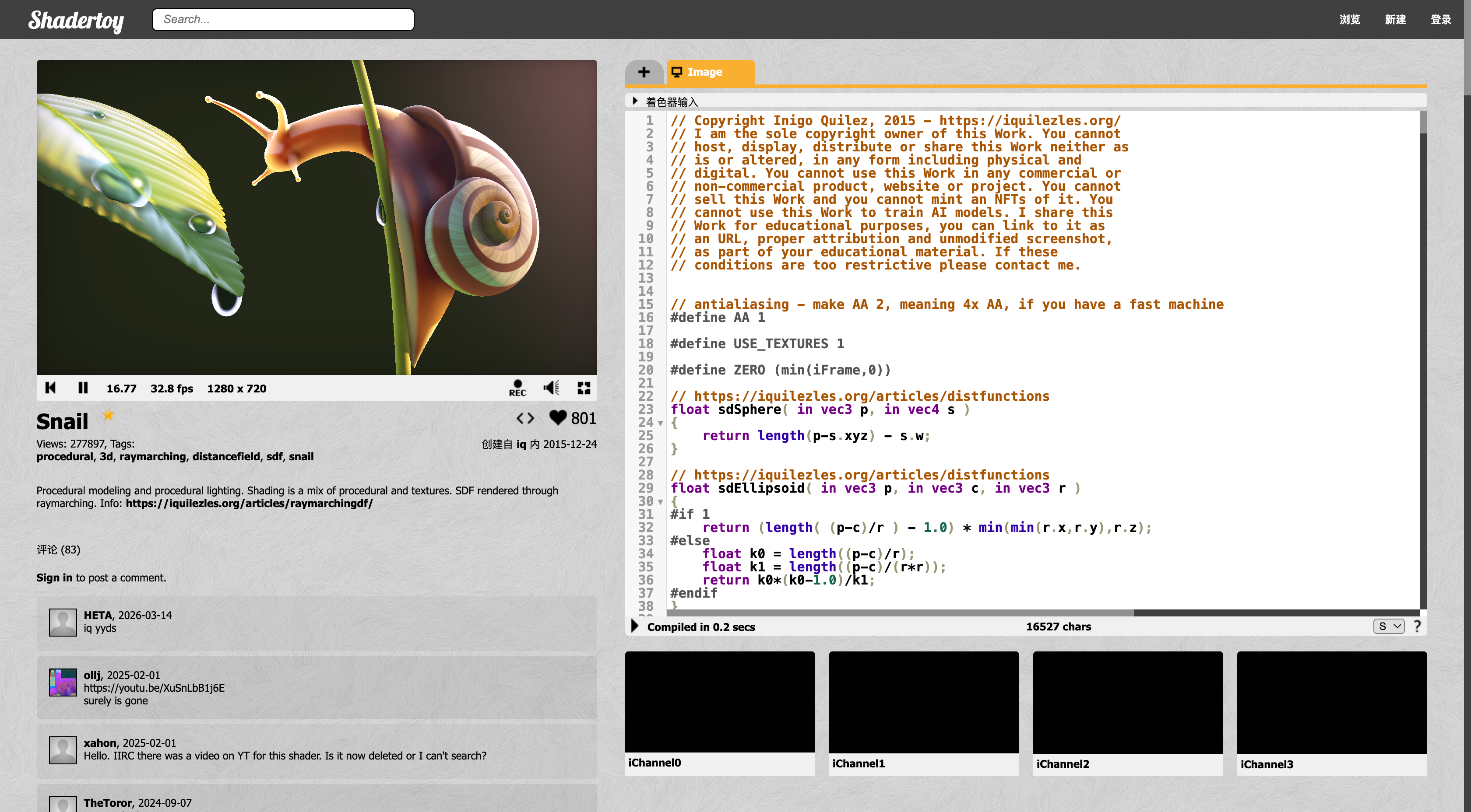
Shadertoy is an online shader playground; the example above is at https://www.shadertoy.com/view/ld3Gz2 . Unfortunately the external video link in the slides is no longer available, so it is not included here.
Game engines already implement many algorithms internally for model rendering, shadows, real-time global illumination, etc., so game developers can focus on gameplay itself rather than the underlying graphics algorithms. But if we want to go deeper into rendering, understanding the principles behind it still matters a lot.
GPU
The GPU (Graphics Processing Unit) is a processor dedicated to graphics pipeline computation. GPUs come in two flavors: discrete and integrated.
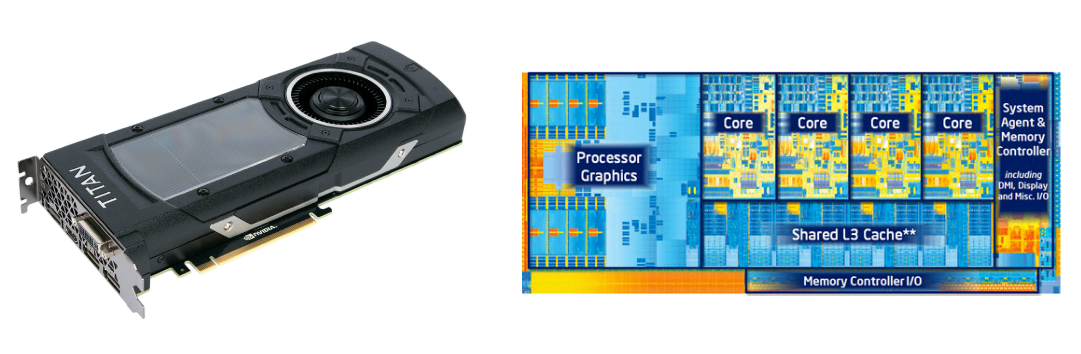
| Trait | Description |
|---|---|
| Heterogeneous multicore | Thousands of parallel processing cores |
| Purpose-built | Optimized for the graphics pipeline |
| Hardware implementation | Algorithms like Z-buffer implemented in hardware |
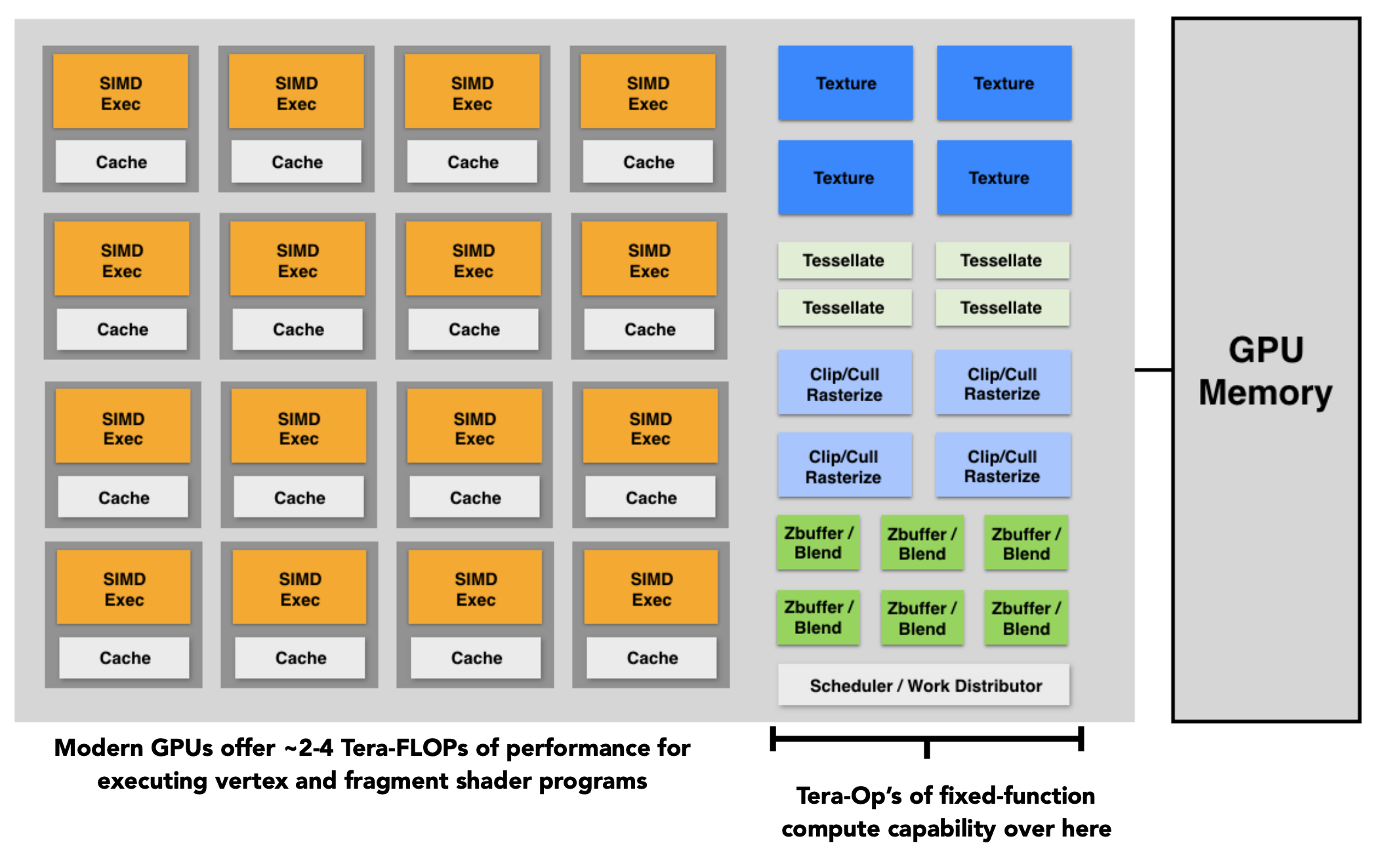
Modern GPU goals: real-time rendering of scenes with hundreds of thousands to millions of triangles, high resolutions (2–4 megapixels + supersampling), 30–60 FPS (higher for VR).
With the rise of AI, GPUs have become the workhorses of large-model computation — thanks precisely to the heterogeneous multicore, massively parallel architecture described above: graphics rendering applies the same computation to millions of vertices and pixels, and LLM training/inference (matrix multiplications, convolutions, attention) decomposes into huge numbers of parallel tasks, fully utilizing thousands of GPU cores. Vendors also designed dedicated hardware and software stacks for AI, such as NVIDIA’s Tensor Cores and the CUDA framework, making GPUs like H100/A100 the primary compute for large models. GPUs were born for graphics yet shine in the AI era — understanding the graphics mindset of “process every pixel/vertex in parallel” is exactly the key to understanding why GPUs accelerate large-model computation so efficiently.
6 Texture Mapping
Why Texture Mapping
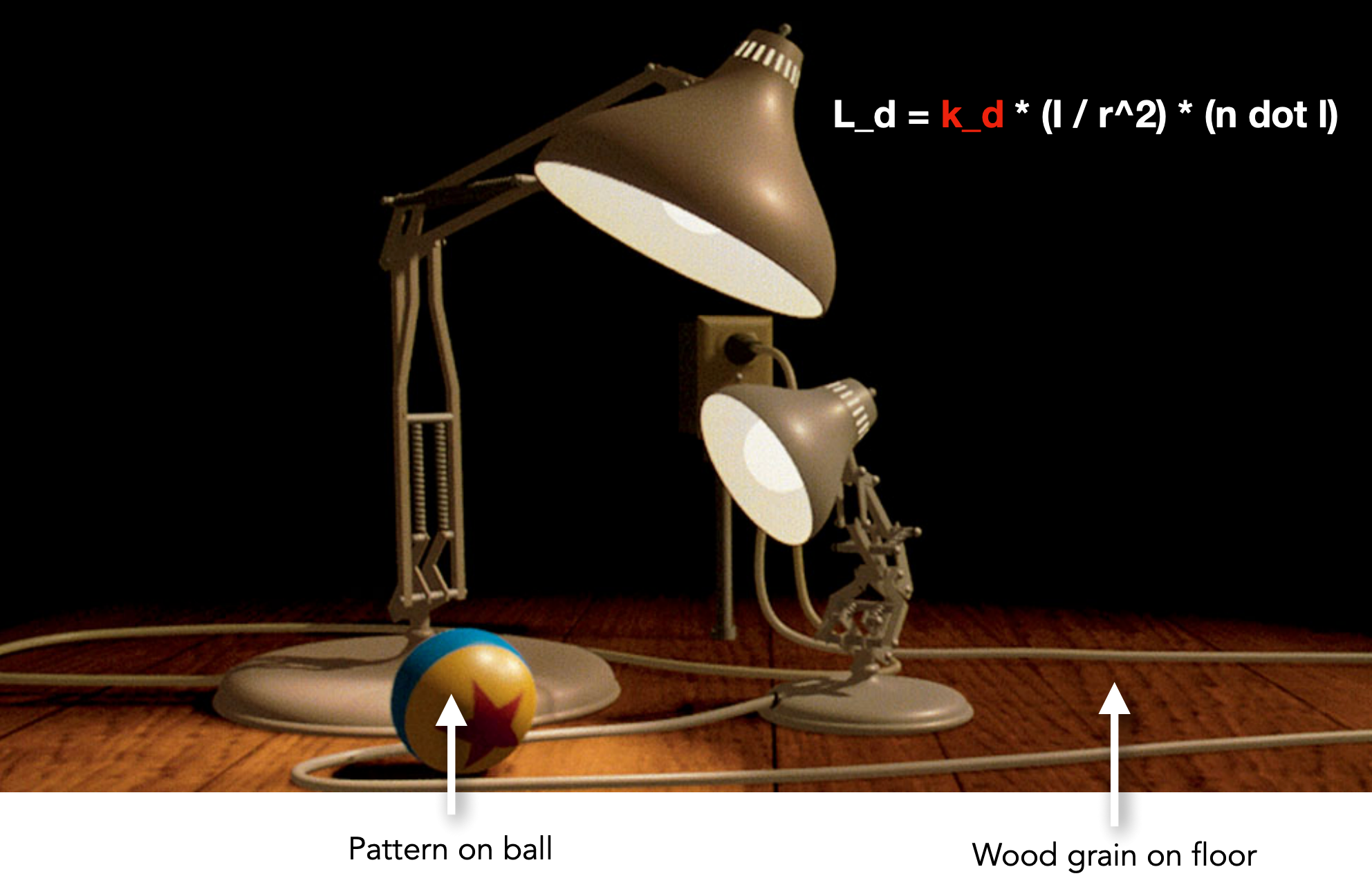
Different positions on a surface should have different colors, but we cannot assign different material properties to every triangle. Texture mapping solves this by “pasting” a 2D image onto a 3D surface.
Basic Principle
Every point on a 3D surface corresponds to a position on a 2D texture image.
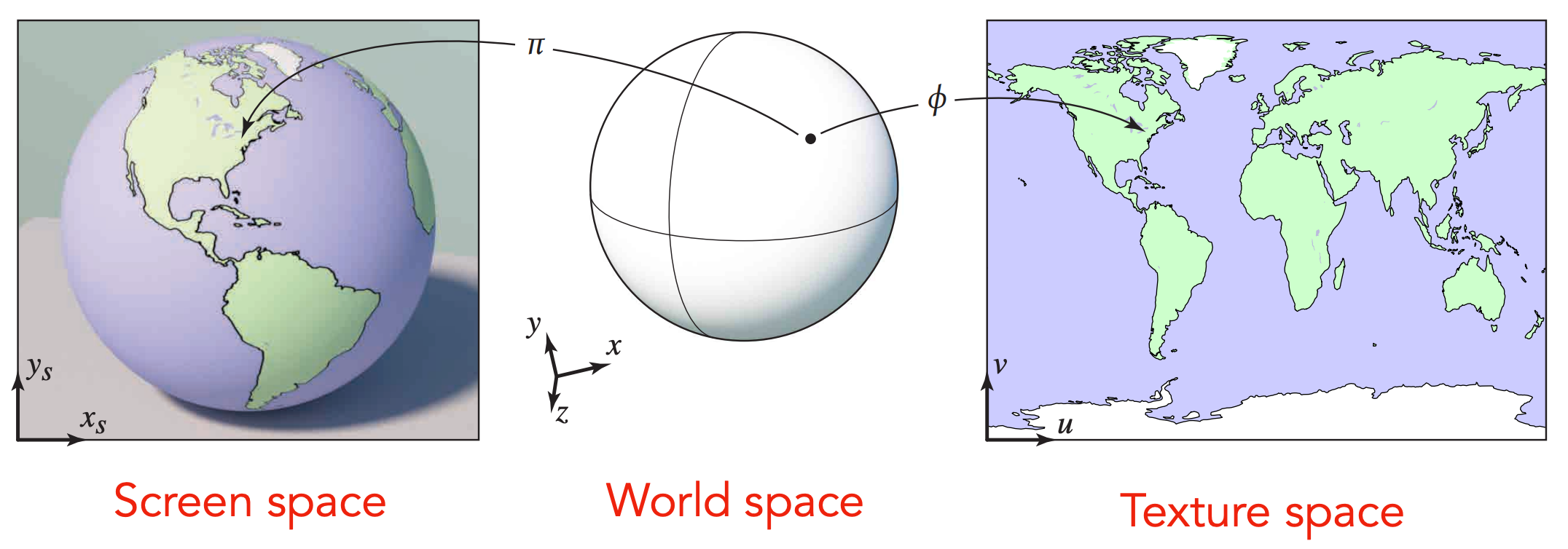
- Every point on a 3D surface has a corresponding location in the 2D texture (image)
- Each triangle “copies” a piece of the texture image onto itself
How to paste an image onto a 3D object:
- Authored by artists/designers.
- Unfold any model onto a plane, keeping the resulting triangles as undistorted as possible, and map triangles onto the texture.
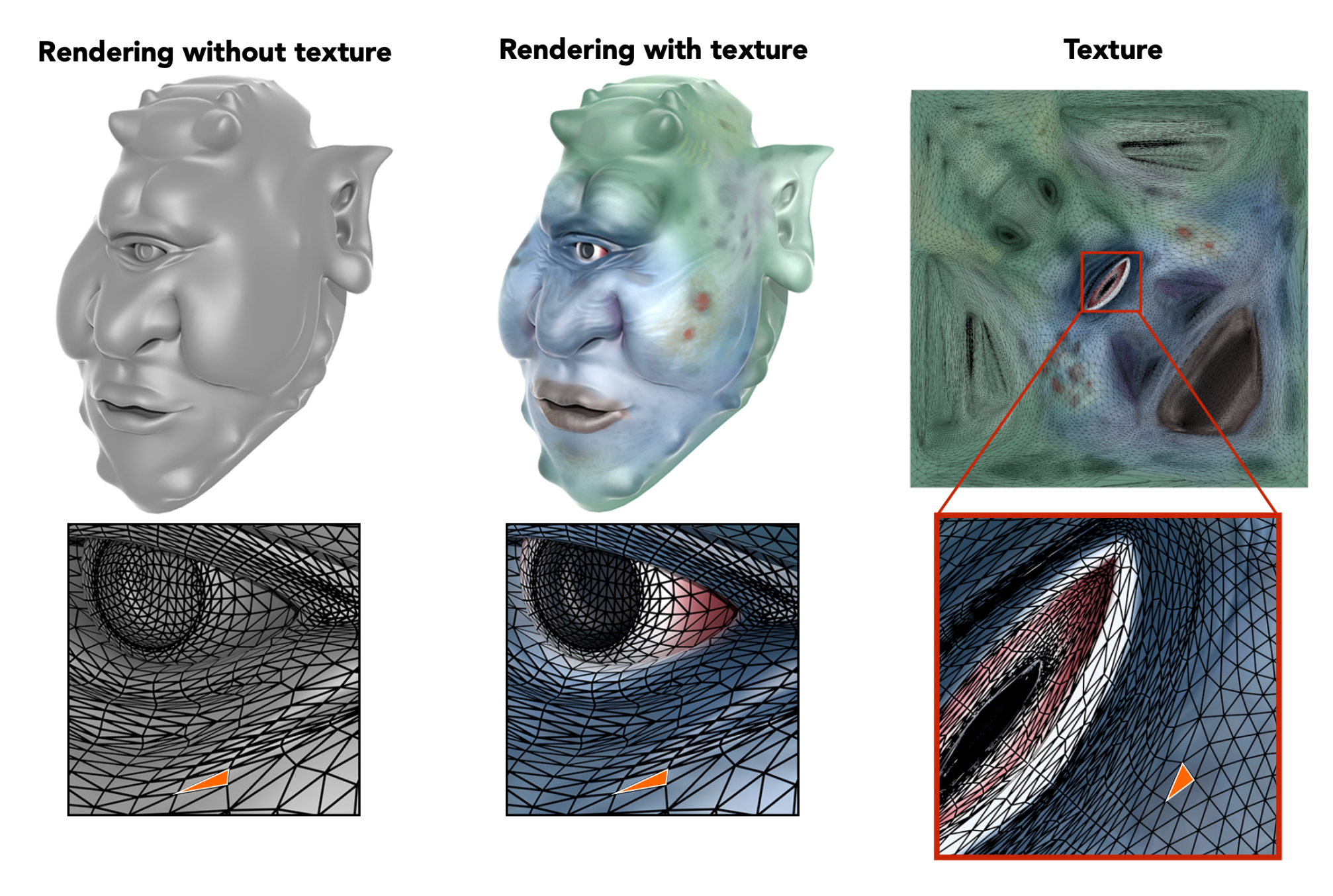
Each triangle vertex is assigned a texture coordinate $(u, v)$, called UV.
UV Coordinates
The way to map an arbitrary triangle onto a texture.
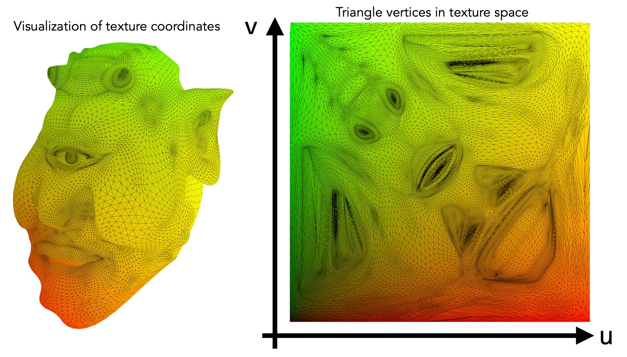
| Property | Description |
|---|---|
| Coordinate range | $u \in [0, 1]$, $v \in [0, 1]$ |
| Visualization | Display $u$ and $v$ as colors to debug texture mapping |
| Texture space | $(u, v)$ defines the location in the texture image |
Reusing Textures
A texture can be applied to any model. The image below uses a single repeated texture — but after repetition, the seams in the middle look abrupt.
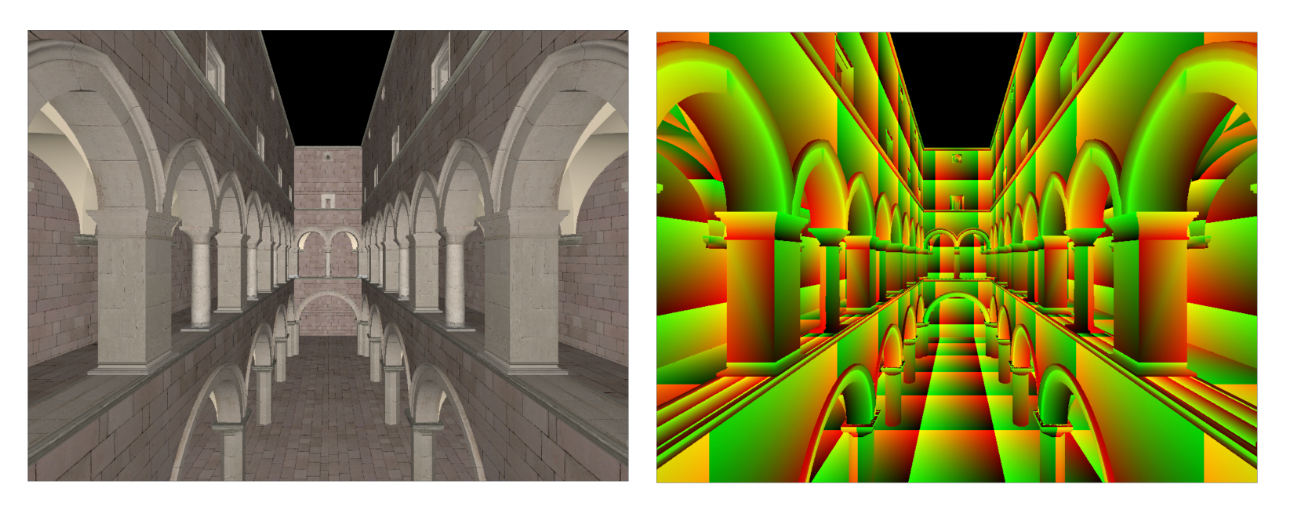
The same texture can be tiled many times over a surface.
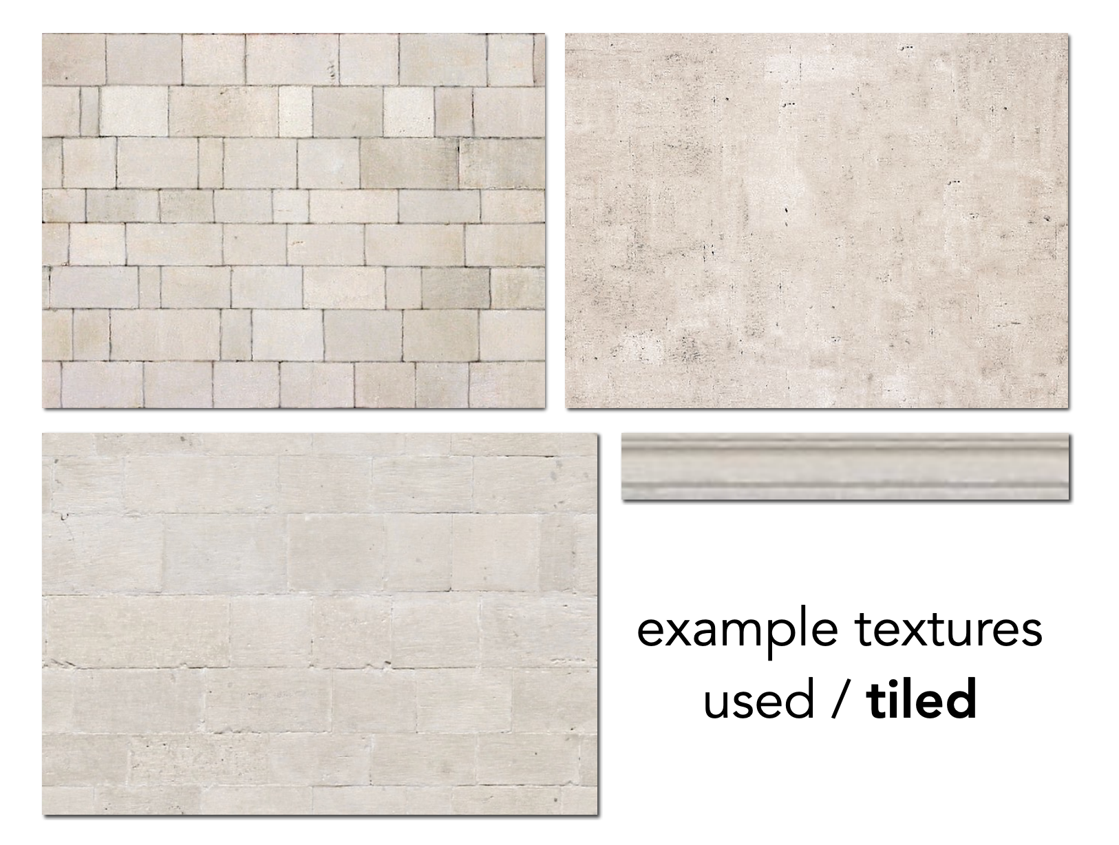
For example a brick wall: one brick texture tiles across the whole wall, saving memory. Seamlessly tileable textures are called “tiled” — very common in game development.
Texture Lookup and Application
Basic flow of applying a texture:
for (each rasterized screen sample (x, y)):        // iterate screen pixels
    (u, v) = evaluate texture coordinate at (x, y)  // interpolate UV via barycentric coords
    texcolor = texture.sample(u, v);                // sample texture color
    set sample's color to texcolor;                 // usually as diffuse coefficient k_d
The texture color is typically used as the diffuse coefficient $k_d$ (diffuse albedo) in the Blinn-Phong model.
7 Barycentric Coordinates
Why Interpolation
We interpolate inside triangles to:
| Question | Answer |
|---|---|
| Why interpolate | Get values specified at vertices; obtain smoothly varying values inside the triangle |
| What to interpolate | Texture coordinates, colors, normals, etc. |
| How to interpolate | Using barycentric coordinates |
Definition
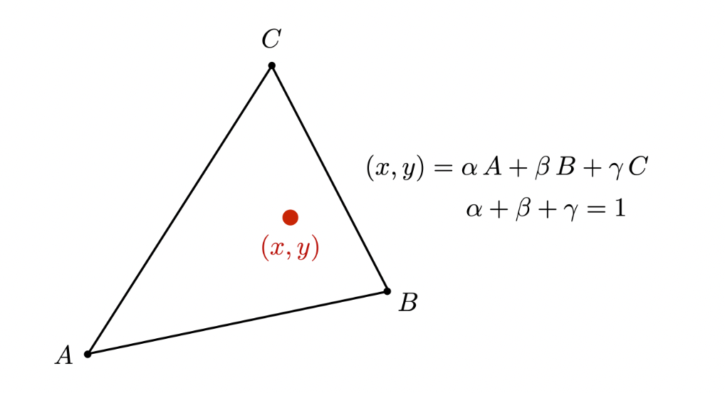
Barycentric coordinates are a coordinate system for a triangle. For triangle ABC and any point $(x, y)$ inside it:
$$ (x, y) = \alpha A + \beta B + \gamma C $$$(\alpha, \beta, \gamma)$ are the point’s barycentric coordinates, satisfying:
$$ \alpha + \beta + \gamma = 1 $$Inside test: the point is inside the triangle when $\alpha \geq 0$, $\beta \geq 0$, $\gamma \geq 0$ — all three nonnegative.
Barycentric coordinates of special points:
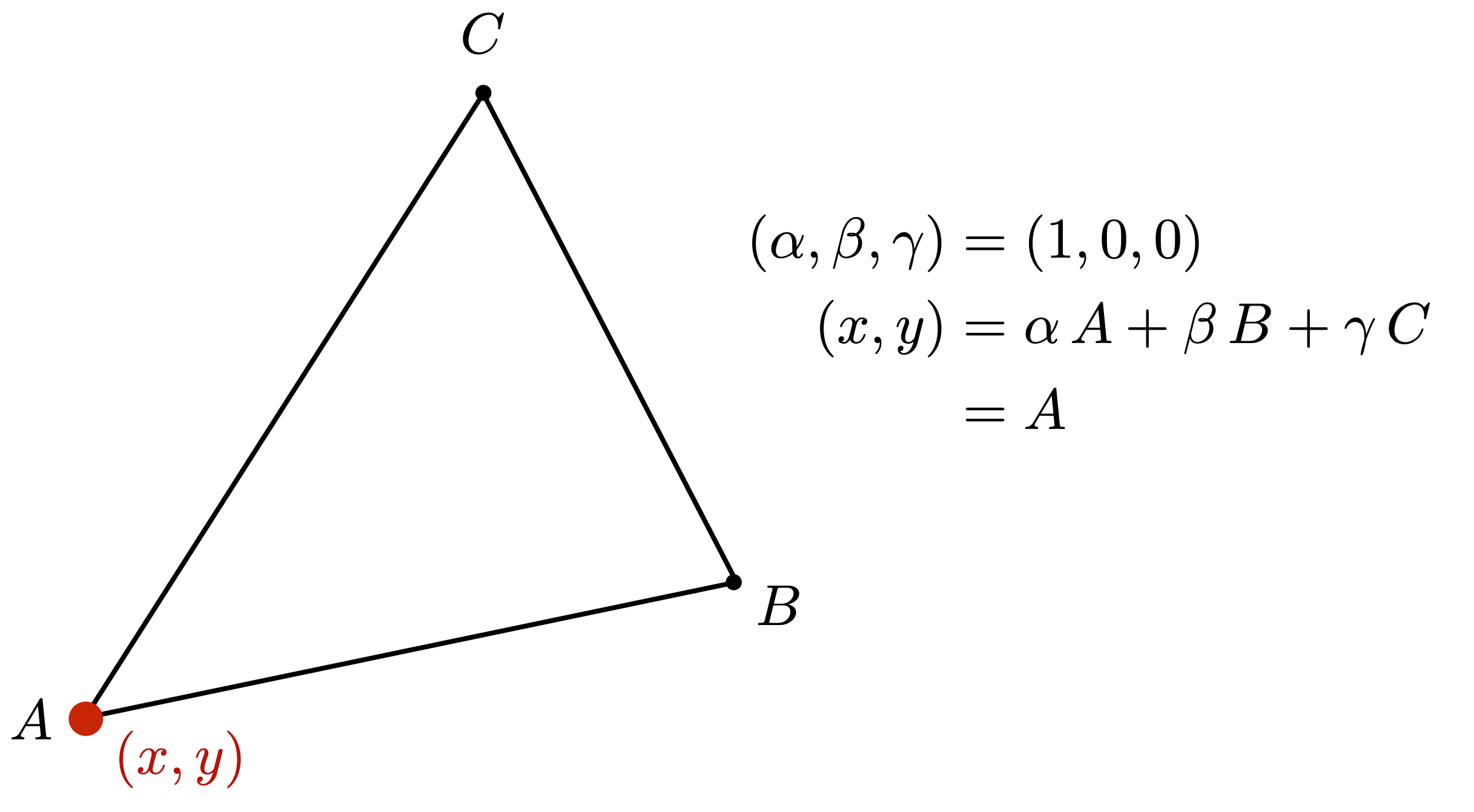
| Point | Coordinates |
|---|---|
| Vertex $A$ | $(1, 0, 0)$ |
| Vertex $B$ | $(0, 1, 0)$ |
| Vertex $C$ | $(0, 0, 1)$ |
| Centroid | $(\frac{1}{3}, \frac{1}{3}, \frac{1}{3})$ |
Geometric Meaning — Area Ratios
Barycentric coordinates can be understood as ratios of sub-triangle areas:
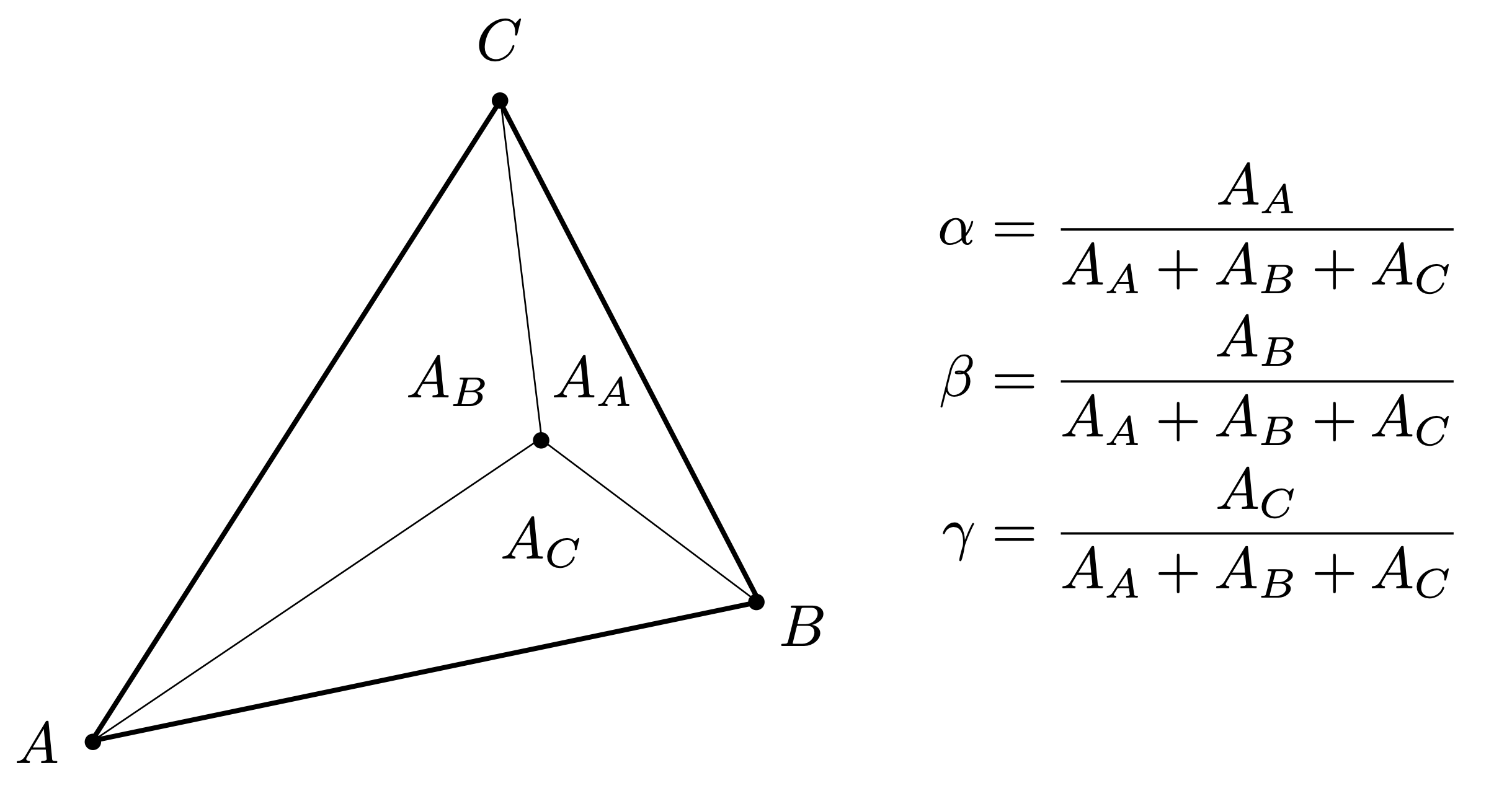
where $A_A$ is the area of the sub-triangle formed by $(x,y)$ and edge BC (opposite to $A$), and so on.
Closed-Form Formula
Given triangle vertices $A(x_A, y_A)$, $B(x_B, y_B)$, $C(x_C, y_C)$ and point $(x, y)$:
$$ \alpha = \frac{-(x-x_B)(y_C-y_B) + (y-y_B)(x_C-x_B)}{-(x_A-x_B)(y_C-y_B) + (y_A-y_B)(x_C-x_B)} $$$$ \beta = \frac{-(x-x_C)(y_A-y_C) + (y-y_C)(x_A-x_C)}{-(x_B-x_C)(y_A-y_C) + (y_B-y_C)(x_A-x_C)} $$$$ \gamma = 1 - \alpha - \beta $$Interpolation in Action
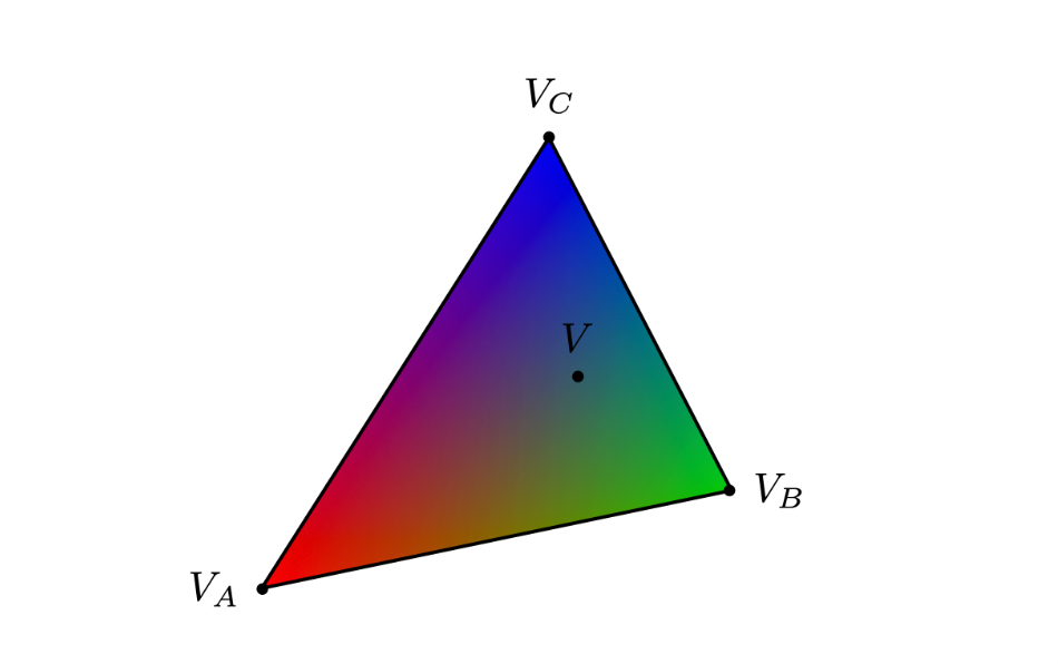
Use barycentric coordinates to linearly interpolate per-vertex values:
$$ V = \alpha V_A + \beta V_B + \gamma V_C $$$V_A$, $V_B$, $V_C$ can be vertex positions, texture coordinates, colors, normals, depths, material properties, etc.
Important caveat: barycentric coordinates are not invariant under projection! Interpolation such as depth must be done in the correct space (3D space) — interpolating depth in screen space generally requires perspective correction.
8 Texture Magnification
Problem: when the texture is too small (insufficient resolution) and must be magnified onto a larger screen region, target pixel locations rarely land exactly on original integer pixel grid points. For example:
- After 2× magnification, which color of the original image does target pixel
(1.5, 2.3)take? - During texture mapping, UV coordinate
(0.37, 0.82)falls between four pixels — which one?
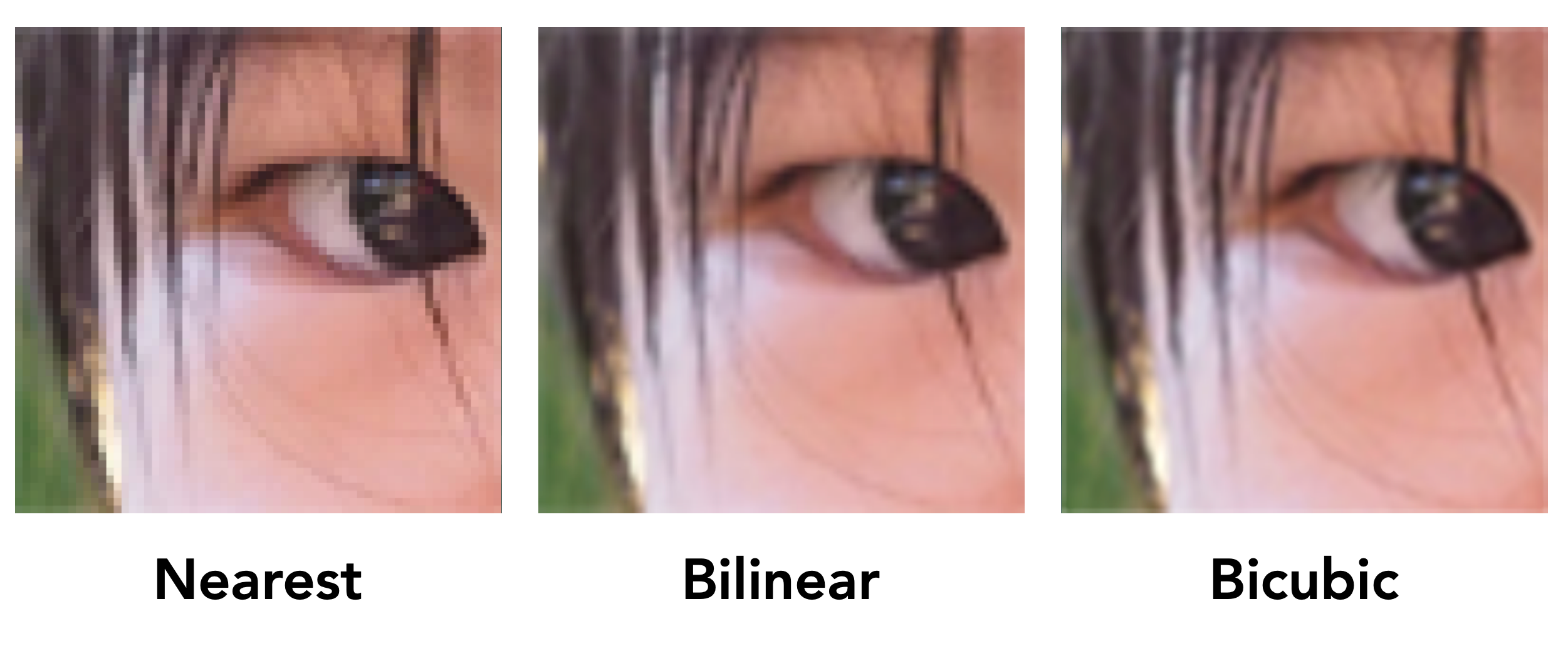
Nearest Neighbor interpolation directly takes the closest integer pixel — simple and brute-force, but produces obvious jaggies and blockiness.
Bilinear Interpolation takes the weighted average of the surrounding 4 pixels, making transitions smoother.
Bilinear uses 4 pixels (first-order polynomial); bicubic uses 16 pixels (third-order polynomial) to fit more complex local surfaces.
Lanczos interpolation is based on the Sinc function (the impulse response of an ideal low-pass filter) — an “upgrade” of bicubic pursuing theoretically optimal reconstruction. (Not covered in the slides, so we won’t dwell on it.)
A pixel of a texture is called a texel (texture element).
Comparison of the Above Methods
| Aspect | Nearest | Bilinear | Bicubic | Lanczos |
|---|---|---|---|---|
| Pixels involved | 1 | 4 | 16 | 36 (Lanczos-3) |
| Polynomial order | 0 (constant) | 1 (linear) | 3 (cubic) | sinc function |
| Continuity | Discontinuous | C⁰ | C¹ | C¹ |
| Edge quality | Jaggies | Blurry | Sharp | Sharpest |
| Ringing | None | None | Slight | Noticeable |
| Cost | 1x | 3x | 10x | 20x+ |
| Typical use | Pixel art | Game textures | Photo upscaling | Professional imaging |
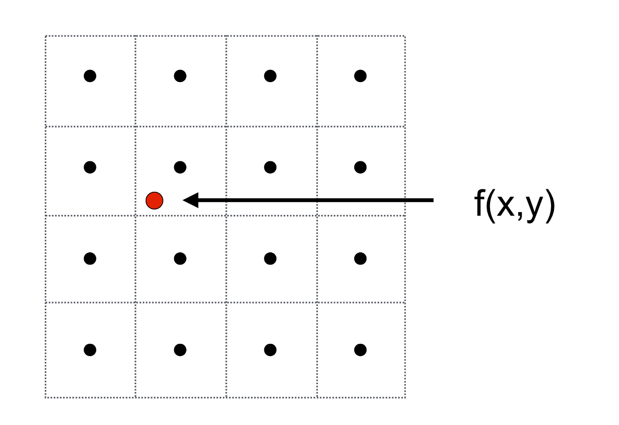
Bilinear Interpolation
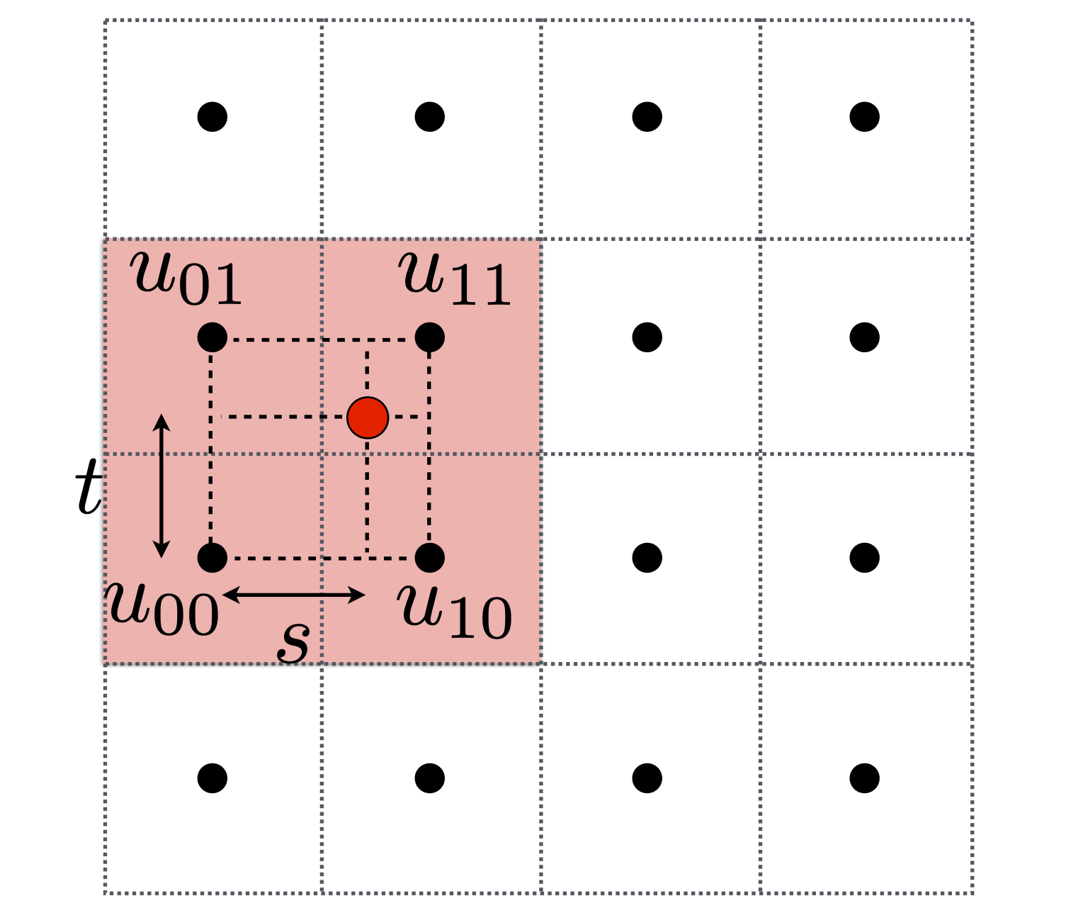
Suppose we want to sample the texture value at the red point $(x, y)$ in a 4×4 texture; the black dots are known texel positions.
Step 1: find the 4 nearest texels $u_{00}$, $u_{10}$, $u_{01}$, $u_{11}$
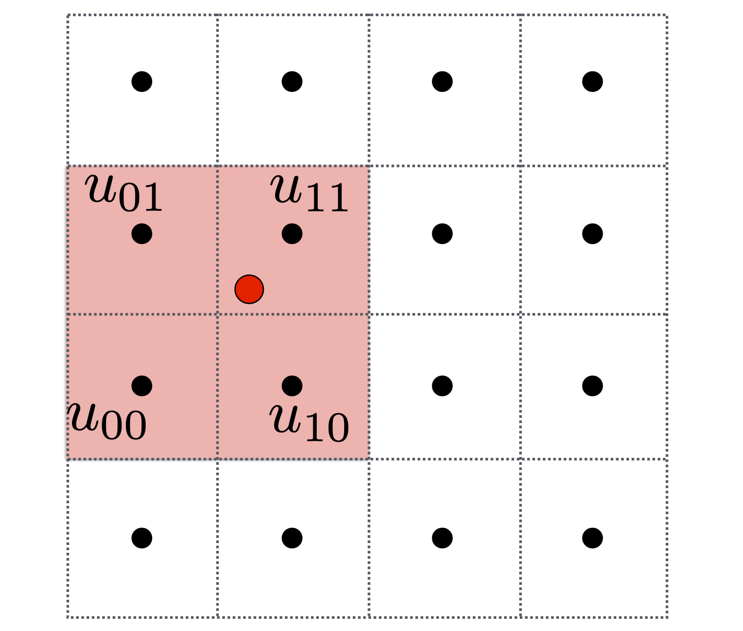
Step 2: compute the fractional offsets $(s, t)$ (position relative to the bottom-left texel, $s, t \in [0, 1]$)
Step 3: define the 1D linear interpolation function:
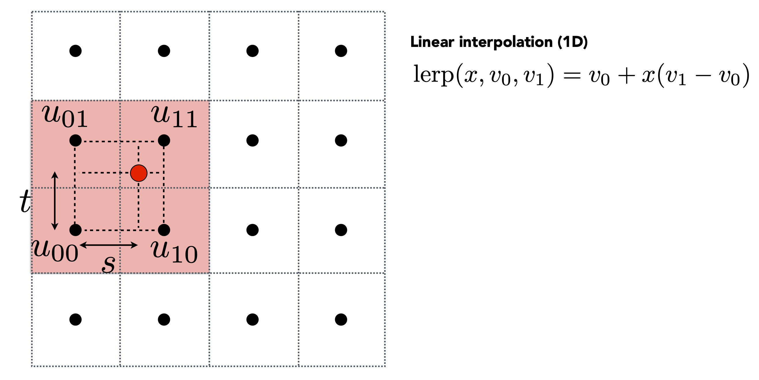
Linear interpolation of $x$ between $v_0$ and $v_1$: when $x = 0$ the result is $v_0$; when $x = 1$ the result is $v_1$.
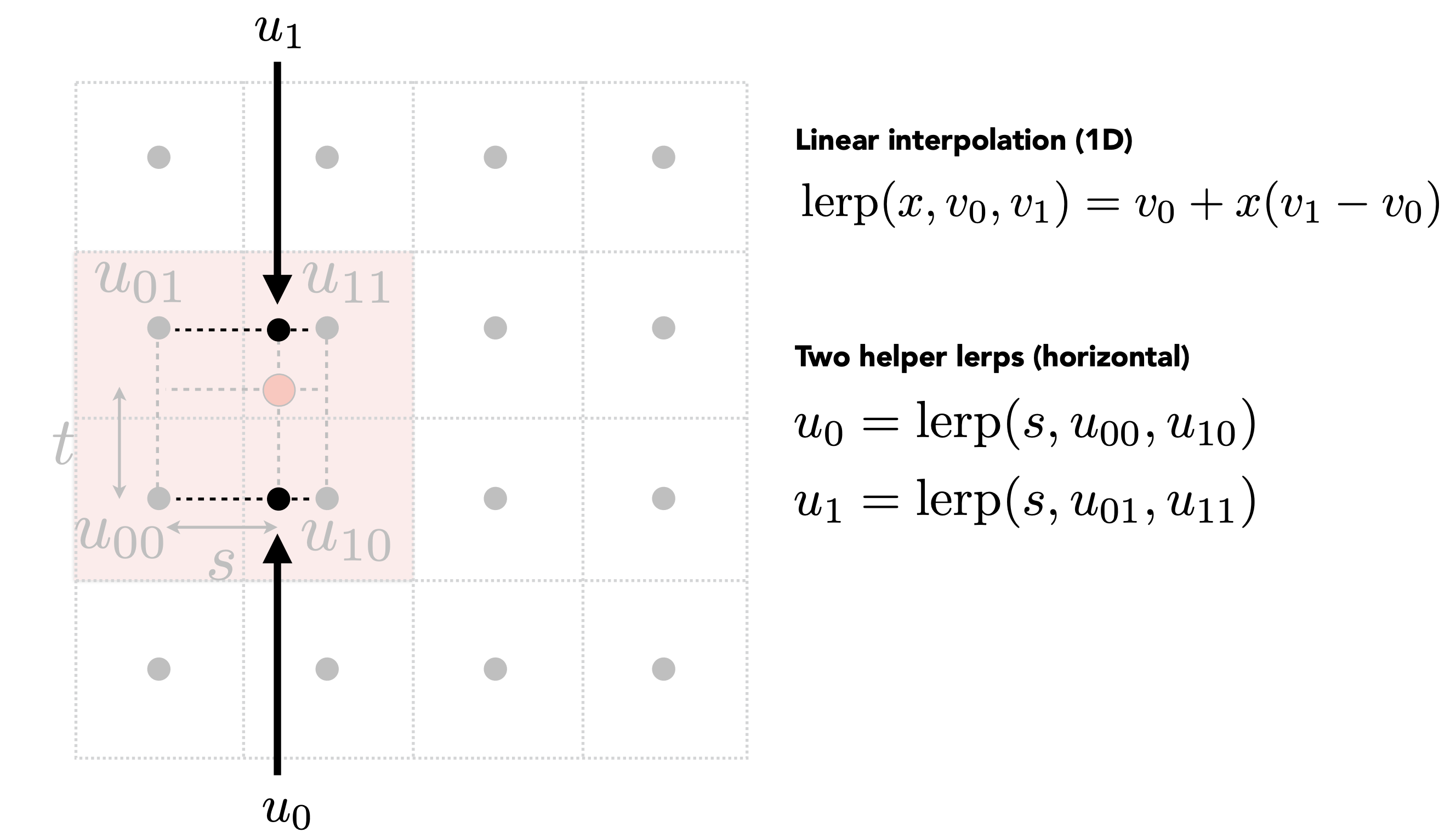
Step 4: two horizontal interpolations:
Step 5: one vertical interpolation between the two horizontal results (final answer):
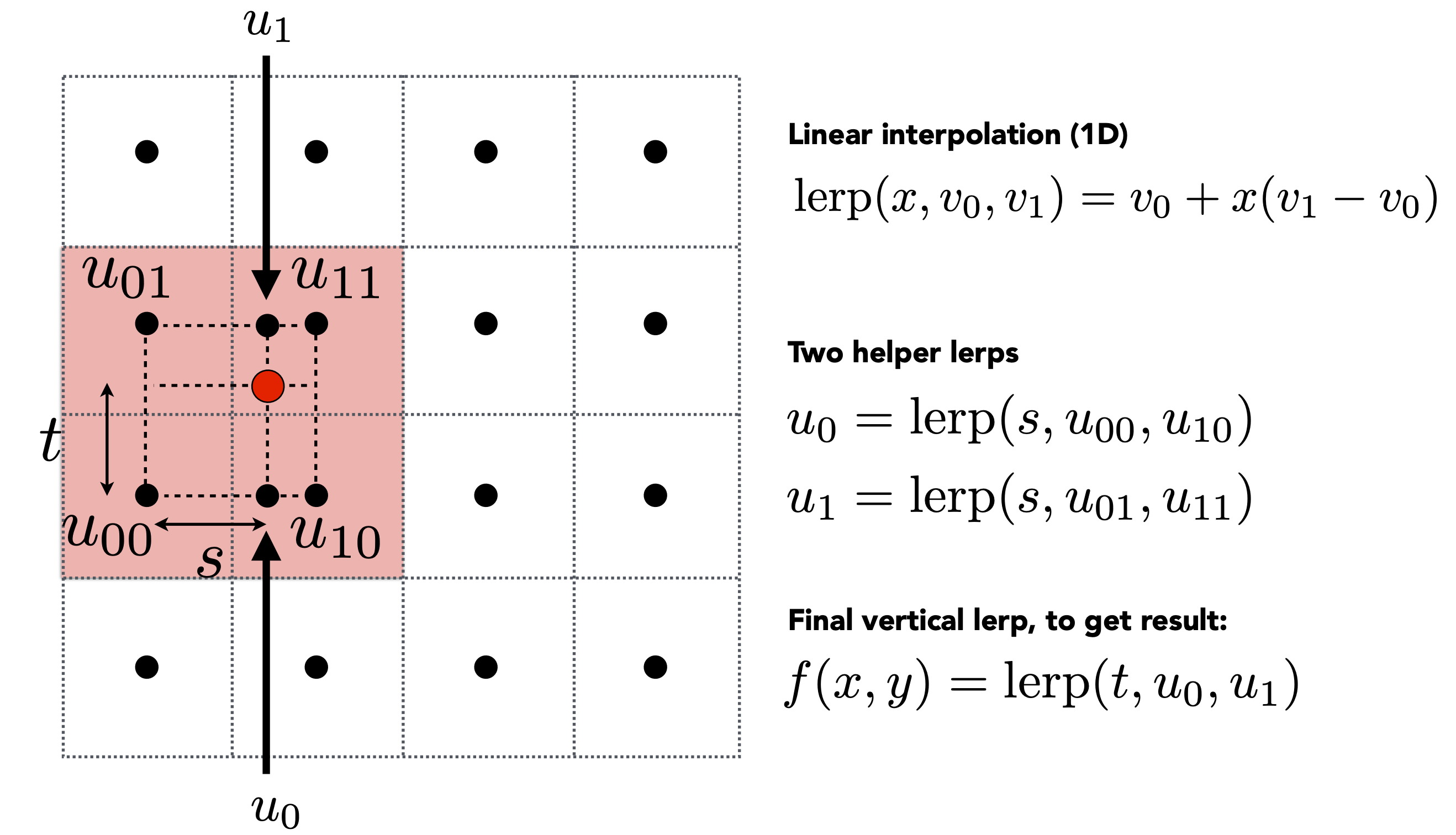
Summary of bilinear interpolation: 3 linear interpolations total (2 horizontal + 1 vertical; horizontal/vertical order can be swapped), achieving good smoothness at reasonable cost.
Bicubic Interpolation
Uses 16 surrounding texels (4×4) and a cubic polynomial. Better quality than bilinear, at higher cost.
9 Texture Minification
Problem: when the texture is too large (too high resolution) and many texels map to one screen pixel, what do we do?
Pixel centroid → texture coordinates → evaluate the texture value.
Problem Analysis
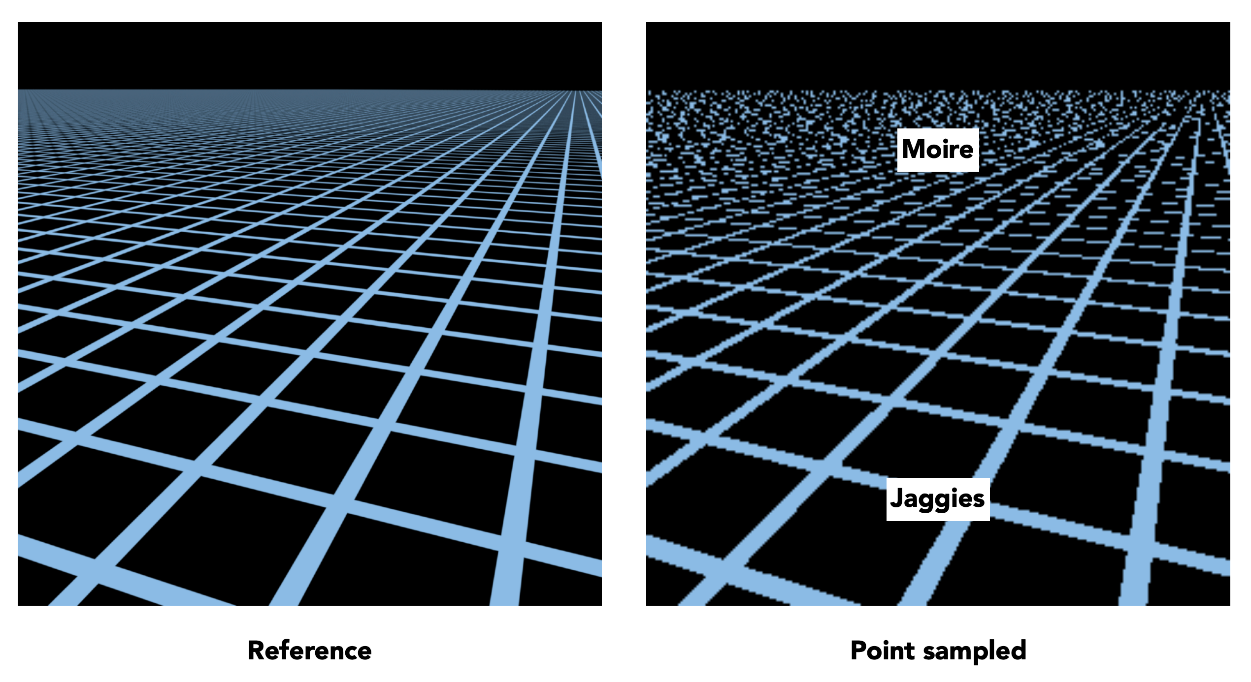
Point sampling causes severe aliasing: Moire patterns and jaggies appear on distant ground textures.
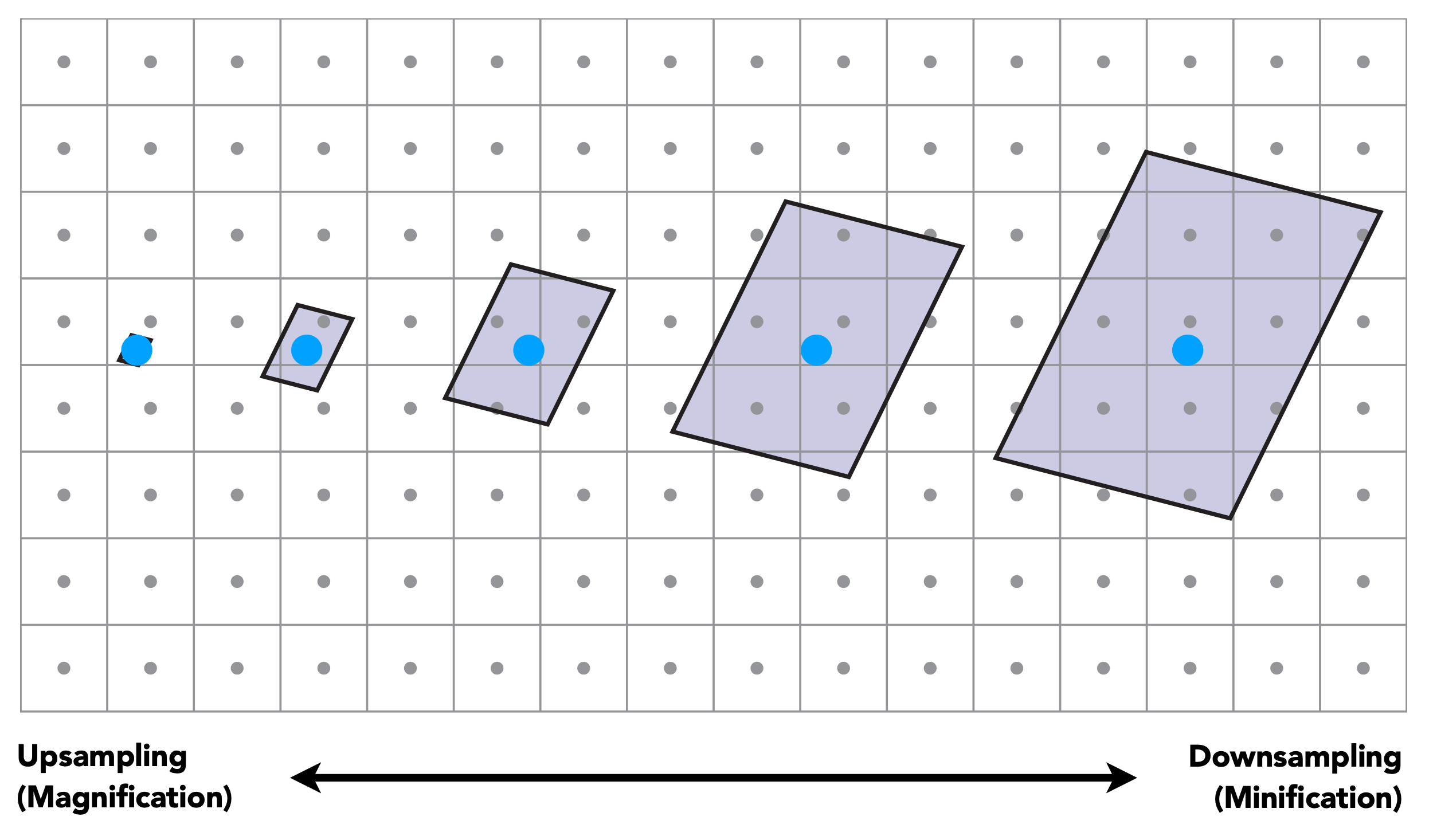
Cause: one screen pixel covers many texels in texture space (the pixel footprint is too large), but point sampling reads only one of them, discarding most of the information.
Limits of Supersampling
Supersampling (e.g. 512x SSAA) can fix aliasing, but:
- Extremely expensive
- When the texture is heavily minified, a single pixel footprint may contain a huge number of texels — the signal frequency is too high and would require even higher sampling rates
A different idea: since the problem is one pixel covering many texels, we don’t need to sample at all — we just need the average over a range.
This is the range query problem:
- Point query: get the texture value at $(u, v)$
- Range query: get the average over the region around $(u, v)$
Mipmap
Mipmap enables fast, approximate, square range queries.
“Mip” comes from the Latin “multum in parvo” — “much in little” (a lot of information in a small space).
Construction
Starting from the original texture (Level 0), halve the side length at each level by averaging 4 adjacent texels:
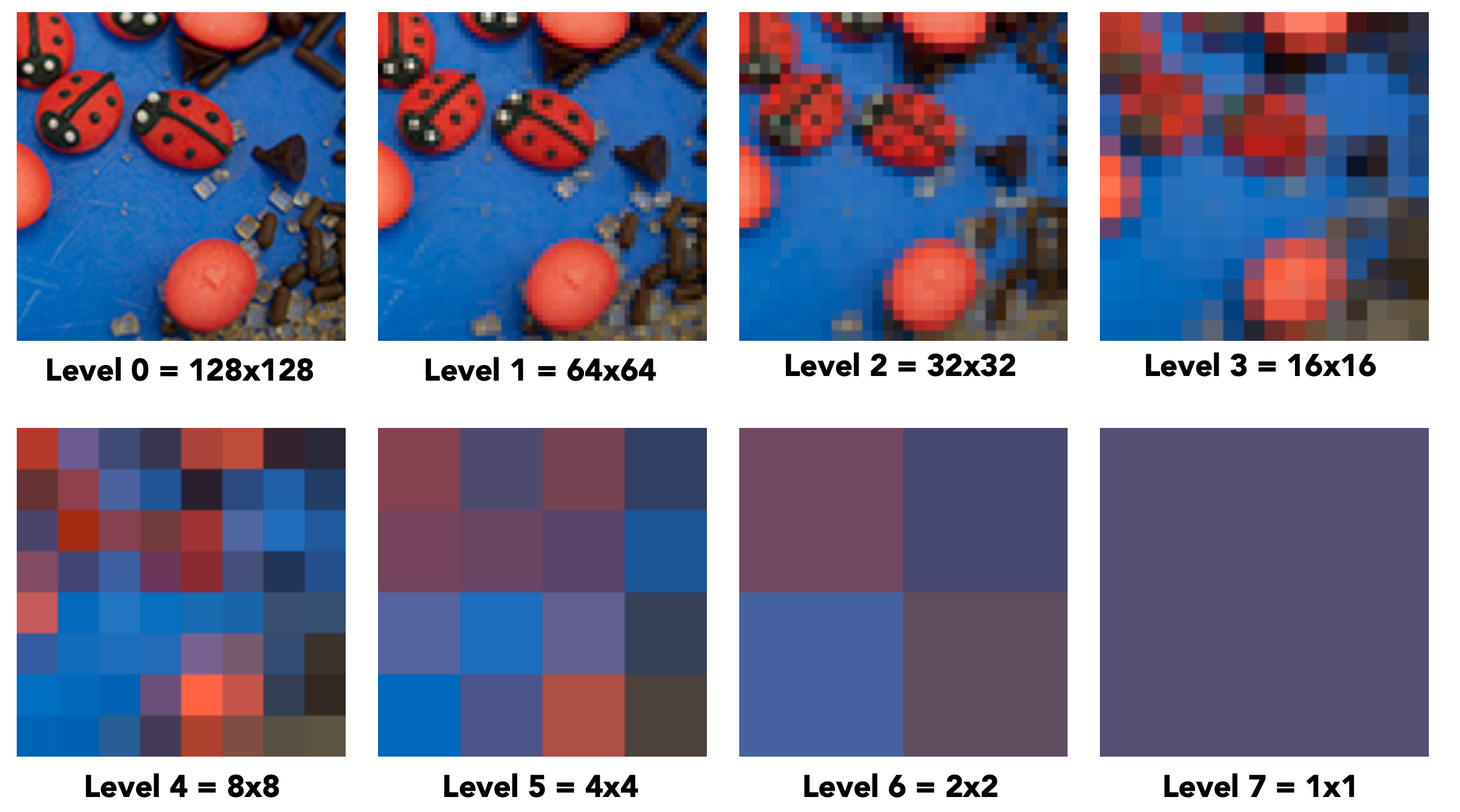
| Level | Resolution | Description |
|---|---|---|
| Level 0 | $128 \times 128$ | Original texture |
| Level 1 | $64 \times 64$ | Average of each 2x2 |
| Level 2 | $32 \times 32$ | Average of each 4x4 |
| Level 3 | $16 \times 16$ | Average of each 8x8 |
| Level 4 | $8 \times 8$ | Average of each 16x16 |
| Level 5 | $4 \times 4$ | Average of each 32x32 |
| Level 6 | $2 \times 2$ | Average of each 64x64 |
| Level 7 | $1 \times 1$ | Global average |
Storage cost: Mipmap adds only $\frac{1}{3}$ of the original texture’s storage.
Derivation: Level 0 is $N \times N$; subsequent levels are $\frac{N}{2} \times \frac{N}{2}$, $\frac{N}{4} \times \frac{N}{4}$, … Sum: $N^2 \cdot (\frac{1}{4} + \frac{1}{16} + \frac{1}{64} + \cdots) = N^2 \cdot \frac{1/4}{1 - 1/4} = N^2 \cdot \frac{1}{3}$ (supplement beyond the slides)
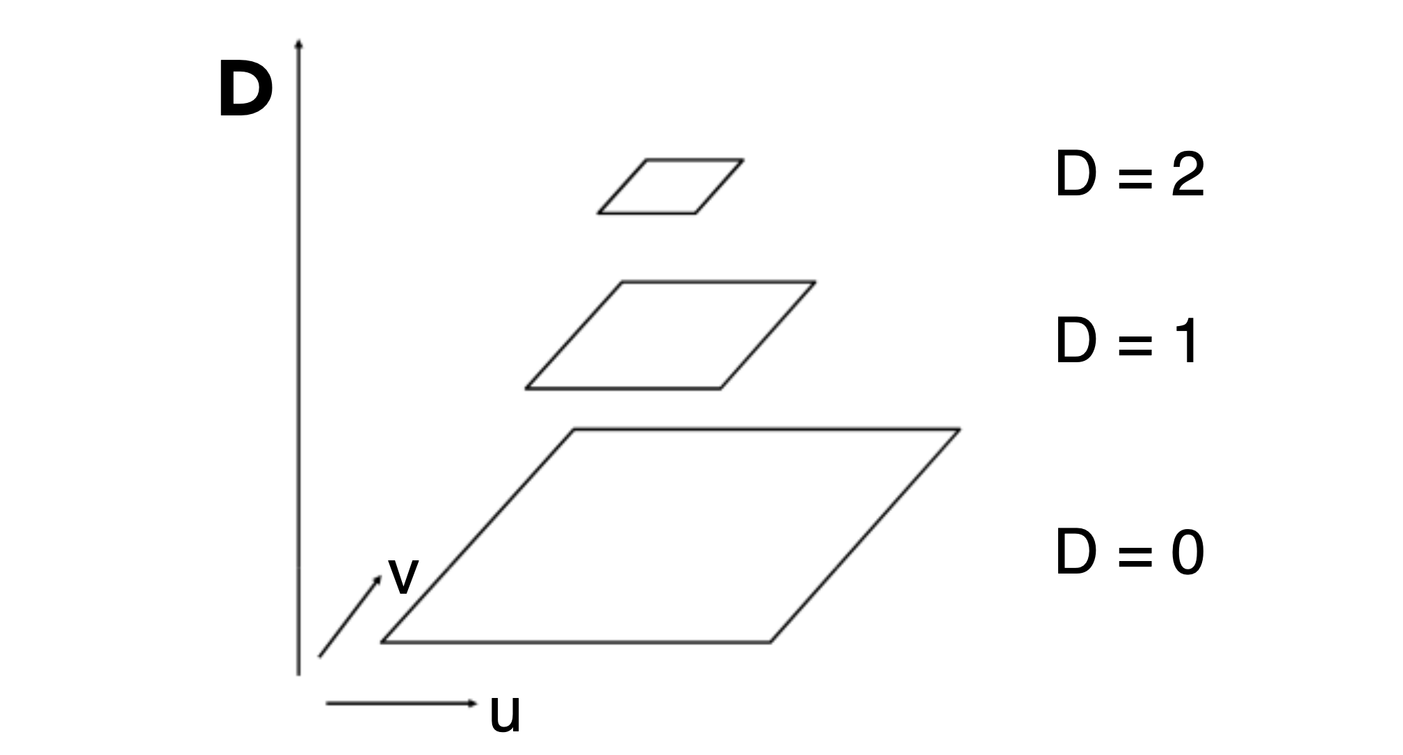
Computing the Mipmap Level D
Pixels at different distances cover different areas in texture space, so the right level must be chosen per location. Near pixels map to tiny texture footprints; far pixels’ footprints are much larger — different pixels have different footprint sizes, so the query range must be estimated per pixel.
Method: estimate the texture footprint size from how fast texture coordinates change between neighboring screen pixels.
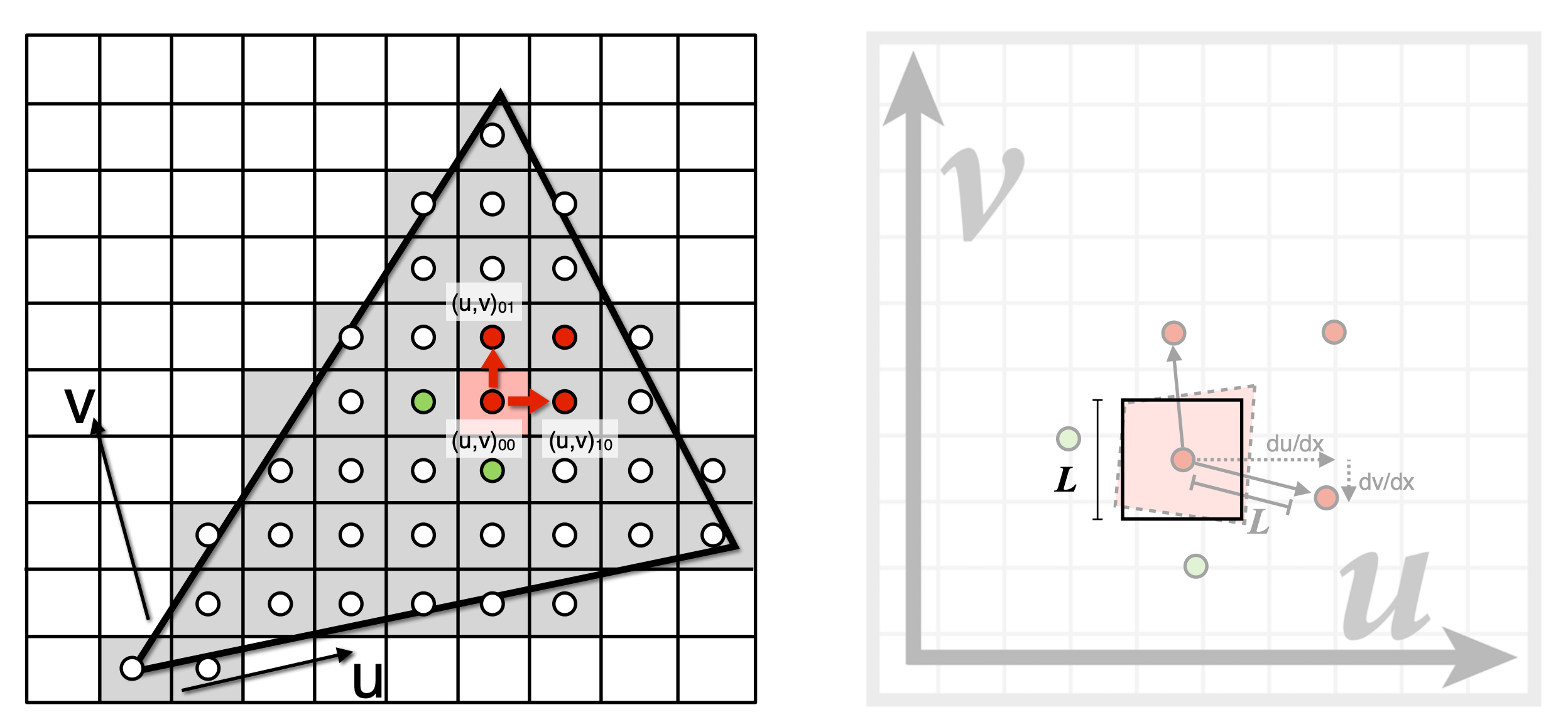
- $L$ approximates the side length of one screen pixel’s coverage in texture space
- $D$ is the corresponding Mipmap level
- $L = 1 \Rightarrow D = 0$ (original texture); $L = 4 \Rightarrow D = 2$ (Level 2)
Mapping the four corners of the square through the inverse transform and measuring the side length works too.
Trilinear Interpolation
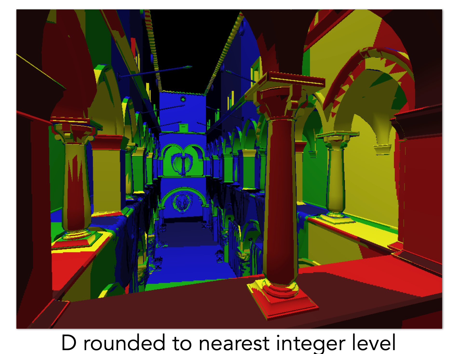
In the scene image above, areas close to us contain lots of detail and need low-level queries; distant areas don’t need that detail and use higher levels. This is a gradual process requiring smooth transitions — hence interpolation.
$D$ is usually not an integer. For smooth results, interpolate linearly between the two neighboring integer levels:
- Bilinear interpolation within Level $\lfloor D \rfloor$ → result $A$
- Bilinear interpolation within Level $\lceil D \rceil$ → result $B$
- Linear interpolation between $A$ and $B$ using the fractional part of $D$
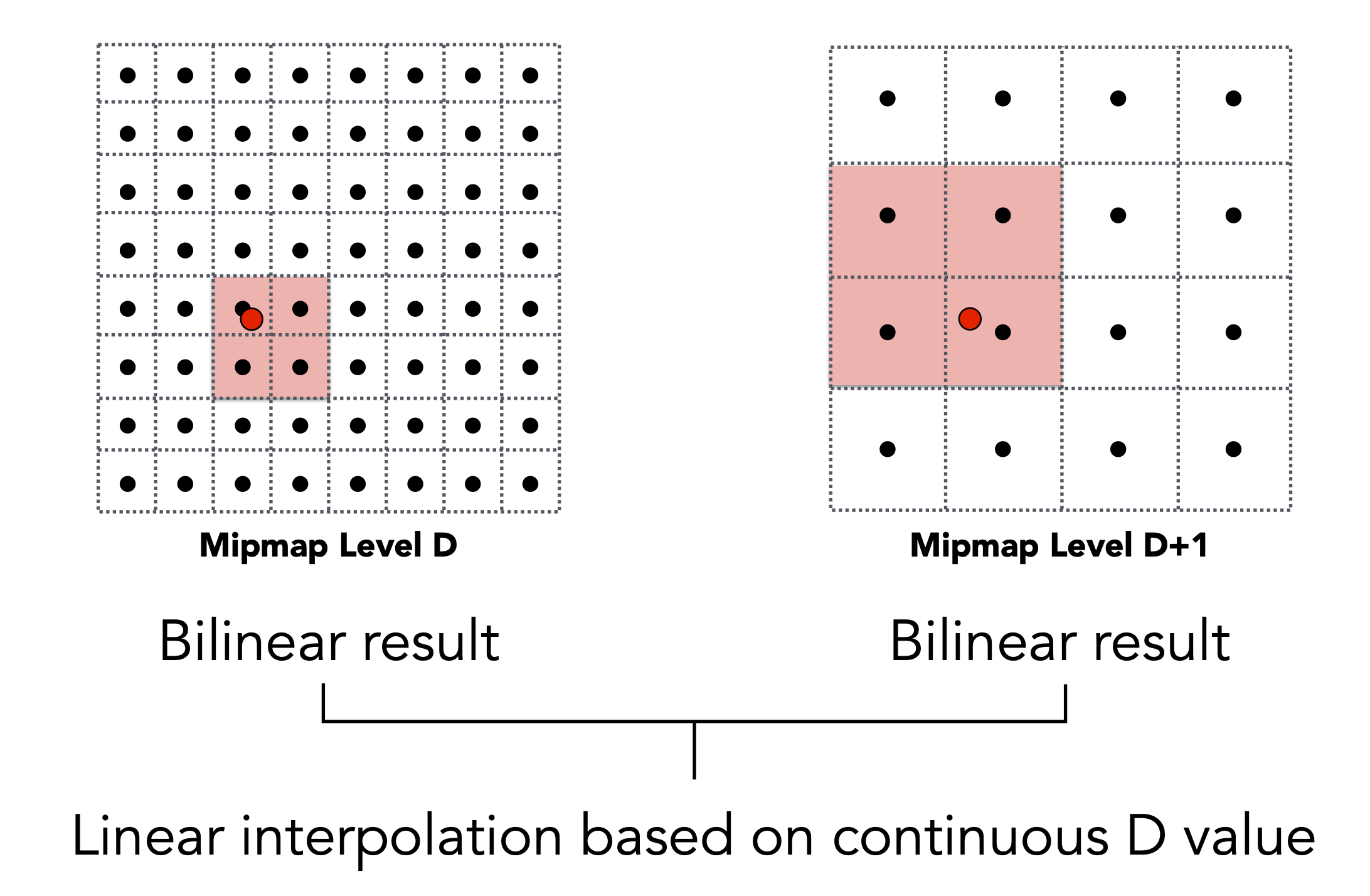
For example, to query level 1.8: bilinearly interpolate inside Level 1 and Level 2 respectively, then linearly interpolate between the two results.
Trilinear interpolation = 2 bilinear interpolations + 1 linear interpolation — smooth results at small cost.
Mipmap Limitation
Mipmap can only query square regions, but actual pixel footprints may be long thin rectangles, causing:
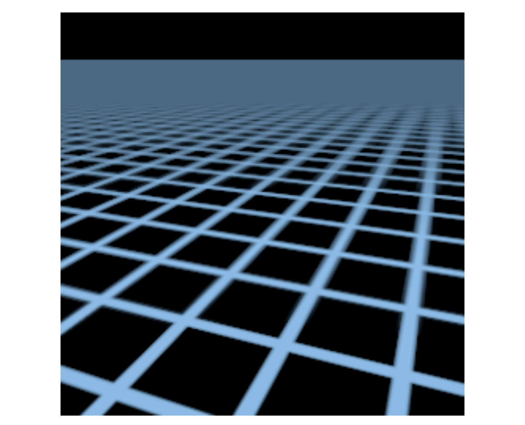
Overblur: Mipmap approximates non-square footprints as squares, averaging over an overly large region, so distant textures become excessively blurry. Anisotropic filtering partially fixes this.
Anisotropic Filtering
Anisotropic filtering handles axis-aligned rectangular region queries, improving on Mipmap.
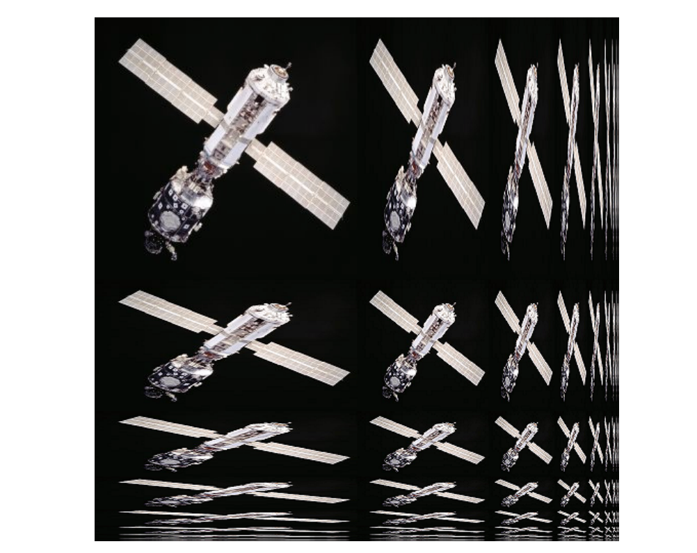
Mipmap essentially halves width and height each level — matching the change of the diagonal square in the figure. Computing different aspect ratios, you can see each column compressed vertically and each row compressed horizontally: compared with Mipmap, there is extra non-uniform horizontal/vertical compression. The shape at column 1, row 3 corresponds to a long thin rectangle when restored to the original image. Such queries let us compute averages over squashed rectangles.
Anisotropic filtering “Nx” corresponds to that many levels: 2x compresses the 2-row 2-column region at the top-left once; 4x compresses the 3×3 region once more.
- Queries averages over axis-aligned rectangles
- Fixes Mipmap’s overblur for such footprints
- Storage cost: needs extra levels at multiple aspect ratios — about 3× the original texture (supplement beyond the slides)
- Limitation: diagonal, skewed footprints remain a problem
“Anisotropic” means behaving differently along different directions; identical behavior in horizontal and vertical directions is “isotropic.”
Irregular Pixel Footprints
A screen pixel’s footprint in texture space can be an irregular shape (especially at oblique viewing angles):
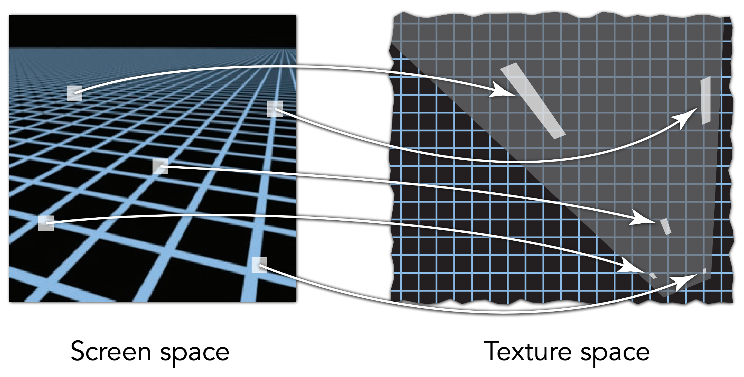
But for the diagonal skewed region above, anisotropic filtering’s axis-aligned rectangles cannot cover it exactly — hence EWA filtering.
EWA Filtering (Elliptical Weighted Average)
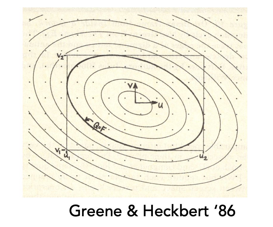
- Uses multiple lookups and weighted averaging
- Approximates the pixel footprint with an ellipse
- Handles irregular footprint shapes
- Mipmap levels still help (accelerating queries)
- Highest cost, best quality
10 Texture Applications
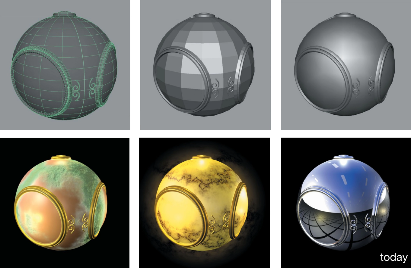
Textures can store more than color — they can store all kinds of data that affect rendering. On modern GPUs, texture = storage + range query (filtering), a general way to bring data into fragment computation.
Environment Mapping
Use textures to store environmental lighting information to simulate reflections.
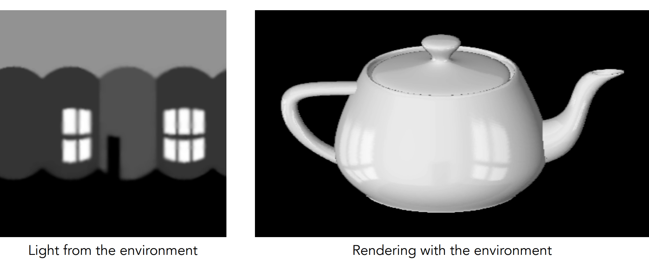
Spherical Environment Map

- Maps the environment onto a sphere
- Problem: severe distortion near the poles
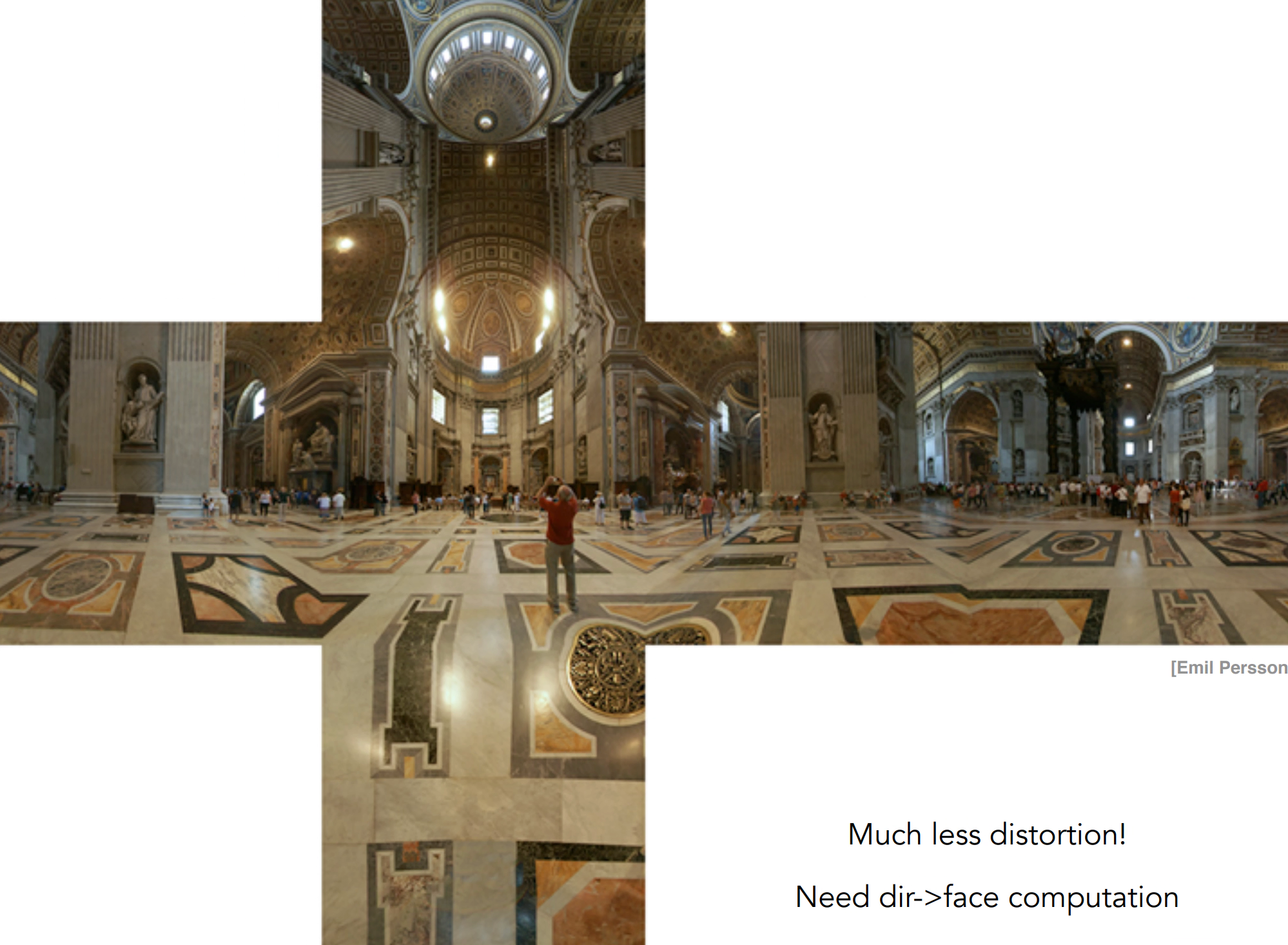
Cube Map
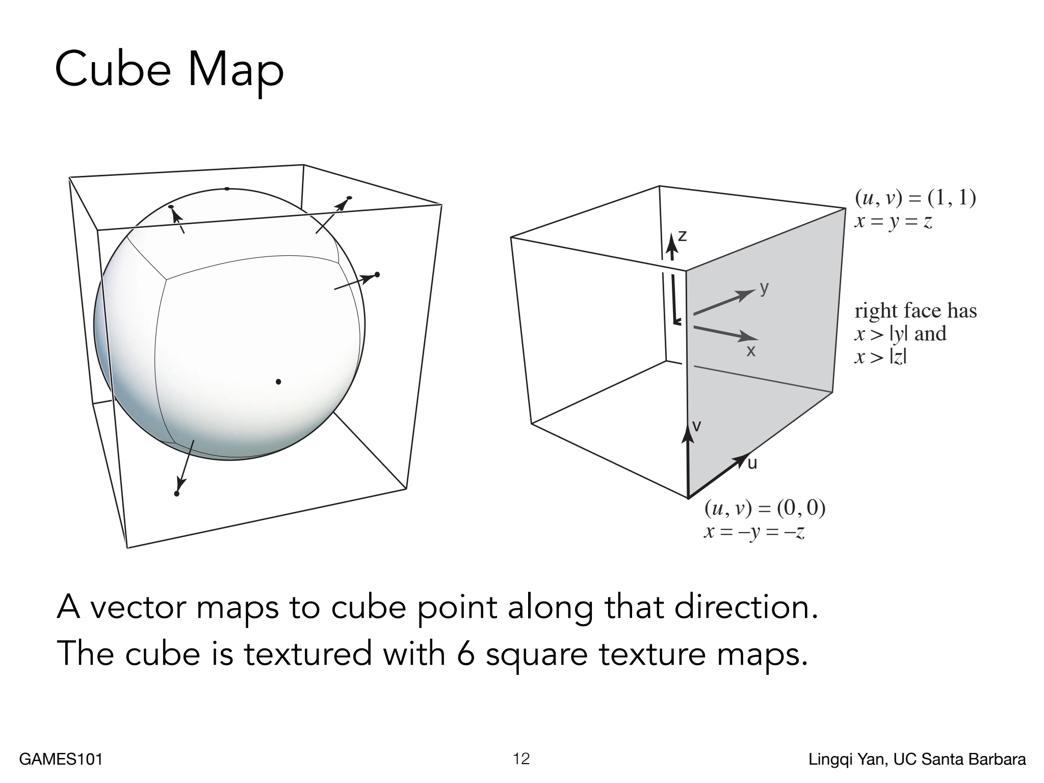
- Maps the environment onto the 6 faces of a cube
- Advantage: less distortion, uniform in all directions
- Usage: a direction vector maps onto a point on the cube; the sampled face and coordinates are determined by the reflection direction (requires dir → face computation)
Bump / Normal Mapping
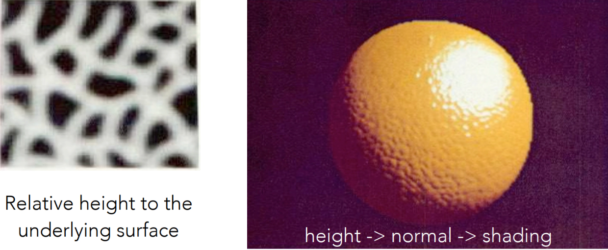
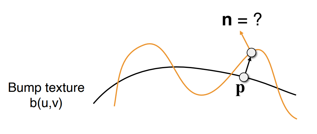
Textures don’t only define color — they can define any attribute. They can specify how far the surface moves up or down along its normal; in the image above, treat black as 0 and white as 1. No need to redefine model detail — it can be handled by the corresponding texture.
Core Idea
Simulate surface detail by perturbing the normal vector, without adding triangles or changing the actual geometry.
Principle
- The texture stores height changes (bump map) or normal directions (normal map) — “storing height/normals” to fake fine geometry
- Each texel defines a height offset; during shading, the perturbed normal replaces the original one in the lighting computation (used only for shading)
- Does not change the actual geometry (vertex positions stay the same)
- Effect: surfaces look bumpy, but silhouettes remain smooth (because it’s “fake”)
Computing the Normal (2D)
Assume the original normal is $\vec{n} = (0, 1)$ and the bump map defines a height change $h(p)$; the perturbed normal is:
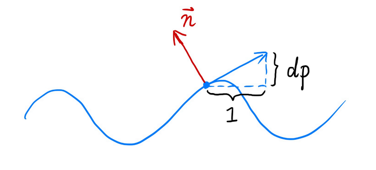
where $dp = c \cdot [h(p+1) - h(p)]$ and $c$ is a constant controlling bump strength.
Get the blue tangent, then the normal perpendicular to it: the tangent moves 1 horizontally and $dp$ vertically, i.e. $(1, dp)$, so the normal is $(-dp, 1)$.
Computing the Normal (3D)
In 3D (original normal $\vec{n} = (0, 0, 1)$), the perturbed normal is:
$$ \vec{n}' = \text{normalize}\left(-\frac{dp}{du}, \; -\frac{dp}{dv}, \; 1\right) $$where $\frac{dp}{du} = c_1 \cdot [h(u+1) - h(u)]$ and $\frac{dp}{dv} = c_2 \cdot [h(v+1) - h(v)]$. Note this formula is defined in a local coordinate frame.
Bump Map vs Normal Map
| Aspect | Bump Map | Normal Map |
|---|---|---|
| Stored data | Height (grayscale) | Normals (RGB channels) |
| Computation | Gradient of height → normal | Read normals directly |
| Precision | Lower | Higher |
Displacement Mapping
Difference from Bump Mapping
| Aspect | Bump Mapping | Displacement Mapping |
|---|---|---|
| Geometry change | None | Vertex positions truly moved |
| Silhouette | Edges stay smooth | Edges show bumps too |
| Shadows | No self-shadowing | Self-shadowing possible |
| Requirement | Any model | Model must be finely tessellated |
| Performance | Fast | Slower |
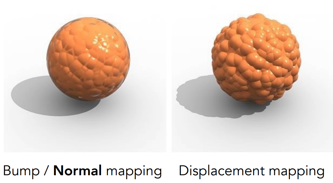
Displacement mapping uses the same texture as bump mapping but actually moves vertex positions, so results are more realistic — at the cost of requiring dense enough triangles, otherwise high-frequency detail cannot be represented.
Shadow Mapping
This topic also corresponds to the Geometry lectures (Lecture 12, second half) — cross-reference them.
Core Idea
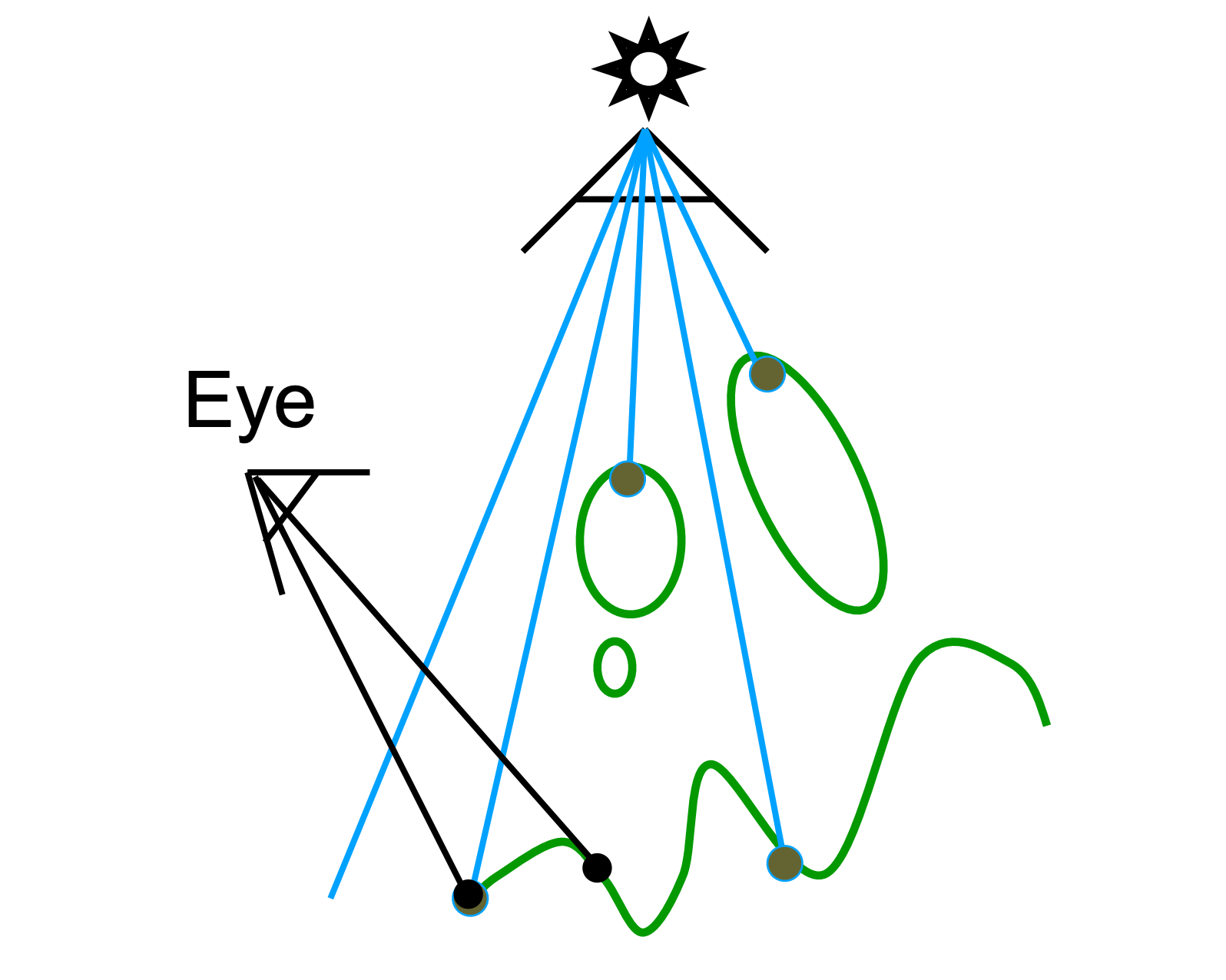
A point is in shadow if it is not in the light’s “line of sight.” This is an image-space, two-pass algorithm: computing shadows needs no scene geometry information, but aliasing artifacts must be handled.
Algorithm Steps
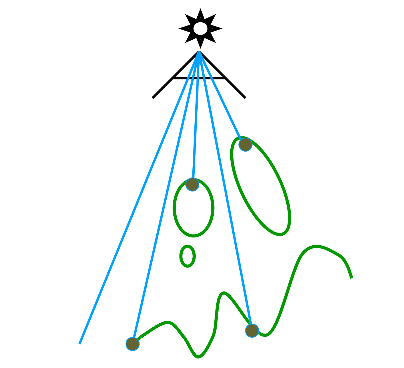
Pass 1: Render from Light
- Put the camera at the light and render the scene
- Record only depth (no color), producing the Shadow Map
- The shadow map stores the nearest depth from the light’s viewpoint (a depth image)
Pass 2: Render from Eye
- Render the scene from the real camera as usual (with depth)
- For each visible point, project it back into light space and compute its depth to the light $d$
- Look up the corresponding depth $d_{\text{shadow}}$ in the shadow map
- Compare: if the depths disagree ($d > d_{\text{shadow}}$), the point is in shadow; otherwise it is not
Shadow Test
| Condition | Conclusion |
|---|---|
| $d \approx d_{\text{shadow}}$ | Not in shadow (the light can see this point) |
| $d > d_{\text{shadow}}$ | In shadow (occluded by another object) |
Shadow Mapping Problems
| Problem | Cause | Solution |
|---|---|---|
| Shadow jaggies | Insufficient shadow map resolution (typical of image-space methods) | Higher resolution maps, cascaded shadows (beyond slides) |
| Shadow acne | Floating-point errors in depth comparison | Add a depth offset (bias) |
| Hard shadows only | Point-light assumption | Soft-shadow algorithms like PCF, PCSS (beyond slides) |
Characteristics
- Pros: no scene geometry needed; purely image-space
- Cons: produces aliasing (limited by shadow map resolution); hard shadows only
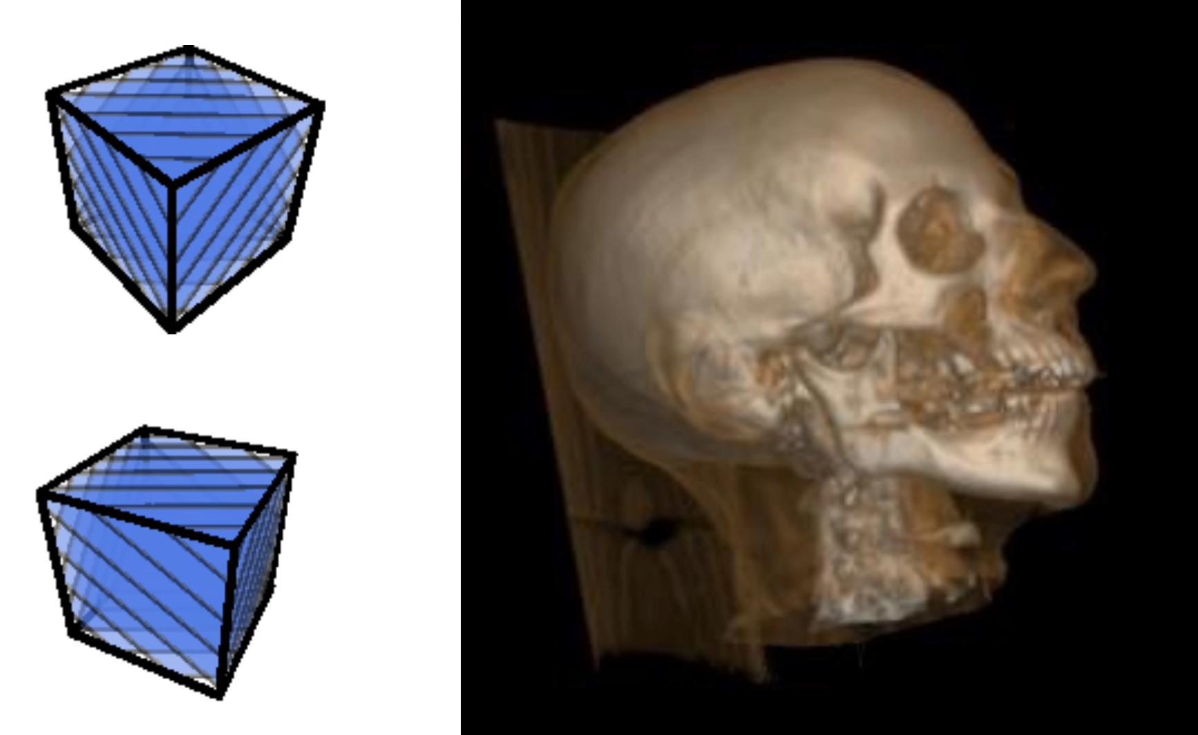
3D Textures and Procedural Textures
3D Texture (Solid Texture)
- The texture is defined throughout 3D space
- Objects look as if “carved” from solid material
- Good for wood grain, marble, etc.
Procedural Texture
- No stored image — texture values are computed by functions (e.g. Perlin noise)
- Saves storage
- Can be infinitely detailed
- Commonly uses noise functions (e.g. Perlin Noise)
Precomputed Shading and Volume Rendering
- Precomputed Shading / Ambient Occlusion: textures can also store precomputed shading results — e.g. an AO map records how occluded each location is from the environment; compositing it lets simply-shaded scenes show rich lighting detail

- 3D Textures and Volume Rendering: define properties like density throughout 3D space (e.g. medical CT data), then sample and integrate along the view ray to render human tissue, smoke, etc. (Marc Levoy’s classic work)
Other Texture Applications
| Application | Description |
|---|---|
| Lightmaps | Store precomputed global illumination |
| Detail maps | Overlay fine detail on base textures |
| Lookup tables (LUT) | Store precomputed lighting lookup tables |
11 Review & Self-Check
What advantages does the Z-buffer have over the painter’s algorithm, and why does it need no sorting?
The Z-buffer maintains a per-pixel minimum depth independently, doing depth tests and updates sample by sample; triangles don’t depend on each other or on drawing order, so no global depth sort is needed (the painter’s algorithm must sort and fails on cyclic occlusion). Time complexity drops to $O(n)$.
Why is Blinn-Phong shading “local,” and why can’t shading produce shadows?
Shading evaluates only the point’s own $\vec{v}$, $\vec{n}$, $\vec{l}$ and material parameters; it has no knowledge of other objects, so it cannot test “is this point visible from the light.” The ambient term merely approximates dark areas. Real shadows require additional visibility computation (e.g. shadow mapping).
What is the half vector $\vec{h}$ for? How does exponent $p$ affect highlights?
$\vec{h} = \frac{\vec{v} + \vec{l}}{\|\vec{v} + \vec{l}\|}$; $\vec{n} \cdot \vec{h}$ measures how close the view direction is to the mirror direction, cheaper than computing the reflection vector. Increasing $p$ narrows the reflection lobe, concentrating the highlight toward a mirror-like look.
Where do Flat / Gouraud / Phong shading compute color, and what is Gouraud’s flaw?
On faces, vertices, and pixels respectively. Gouraud computes color at vertices and interpolates; if a highlight falls inside a triangle rather than at a vertex, it can be lost.
What are the steps of bilinear interpolation? Why is trilinear interpolation needed?
Find the 4 nearest texels → compute offsets $(s,t)$ → two horizontal lerps + one vertical lerp. Mipmap level $D = \log_2 L$ is usually non-integer, so trilinear interpolation does one bilinear query in each of the two adjacent levels, then linearly blends them by the fractional part — removing level-transition seams.
Why does Mipmap cause overblur, and how do anisotropic filtering and EWA address it?
Mipmap only supports square range queries, so a squashed, elongated footprint is approximated by an oversized square average. Anisotropic filtering supports axis-aligned rectangles; EWA approximates arbitrary footprints with ellipses via multiple weighted lookups — best quality, highest cost.
What is the essential difference between bump mapping and displacement mapping?
Bump mapping only perturbs normals without touching geometry (silhouettes stay smooth, no self-shadowing); displacement mapping actually moves vertices, so contours and shadows are correct — at the cost of requiring dense tessellation.
What do the two passes of shadow mapping do? How is shadow acne mitigated?
Pass 1 renders from the light and stores only depth (the shadow map); Pass 2 renders from the camera, projects each visible point back into light space and compares depths — $d > d_{\text{shadow}}$ means shadowed. Shadow acne from floating-point depth errors is mitigated by adding a bias offset.
This post is note #5 in the GAMES101 - Modern Computer Graphics learning series.