- Instructor: Lingqi Yan | UCSB
- Bilibili: https://www.bilibili.com/video/BV1X7411F744
- Lectures covered: Lecture 13 (Ray Tracing 1: Whitted-Style Ray Tracing), Lecture 14 (Ray Tracing 2: Acceleration & Radiometry), Lecture 15 (Light Transport & Global Illumination), Lecture 16 (Ray Tracing 4: Monte Carlo, Path Tracing)
Note: ray tracing is the longest block in GAMES101, spanning lectures 13-18. This post covers lectures 13-16 — from Whitted-style ray tracing, intersection tests and acceleration structures, through radiometry and the rendering equation, to path tracing. Materials and appearances (Lecture 17) and advanced rendering topics (Lecture 18) get their own posts.
Ray tracing is a rendering technique that generates images by simulating how light propagates through a scene. Compared with rasterization, it captures global illumination effects accurately — reflections, refractions, soft shadows, indirect lighting — and is the core technique behind offline rendering for film and animation.
1 Why We Need Ray Tracing
Limitations of Rasterization
Rasterization is fast, but it struggles badly with global effects:
| Effect | Can rasterization handle it? | Notes |
|---|---|---|
| Soft shadows | Hard | Requires computing the penumbra |
| Light bouncing multiple times | No | Rasterization mainly handles direct lighting |
| Specular reflection | No | Requires tracing reflected rays |
| Refraction | No | Requires tracing refracted rays |
| Ambient occlusion (AO) | Hard | Requires geometric occlusion queries |
| Global illumination (GI) | No | Requires simulating multiple bounces |
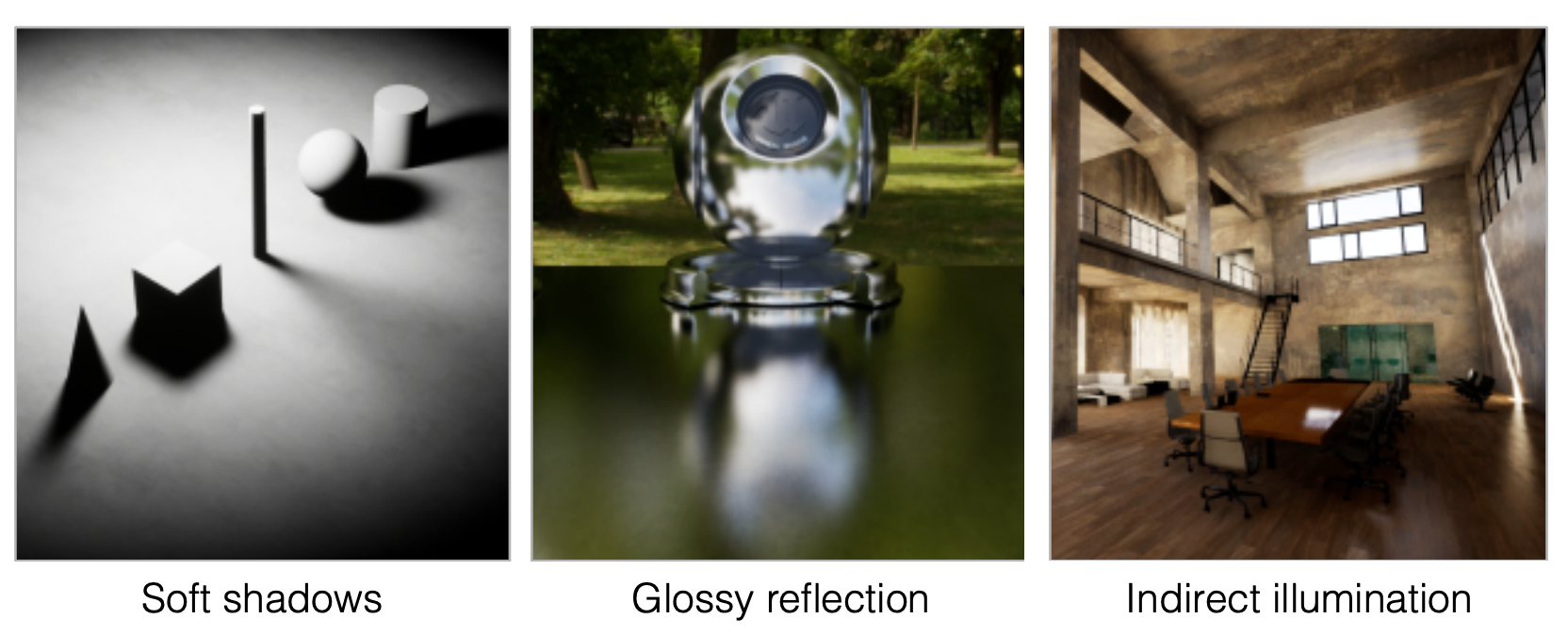
Pros and Cons of Ray Tracing
| Property | Rasterization | Ray Tracing |
|---|---|---|
| Speed | Fast (real-time) | Slow (offline) |
| Quality | Relatively low | High (physically accurate) |
| Global effects | Difficult | Naturally supported |
| Use cases | Games, real-time rendering | Film, animation (~10K CPU core-hours per frame) |
The core problem with rasterization: once light bounces more than once, it can no longer handle the situation correctly. Ray tracing solves this by recursively tracing light paths.
2 Basic Concepts of Light Rays
Three Assumptions About Rays
- Light travels in straight lines (not strictly physically correct)
- Rays do not collide with each other (not strictly physically correct)
- Light travels from the light source to the eye (the physics is invariant under path reversal — reversibility)
Emission Theory of Vision
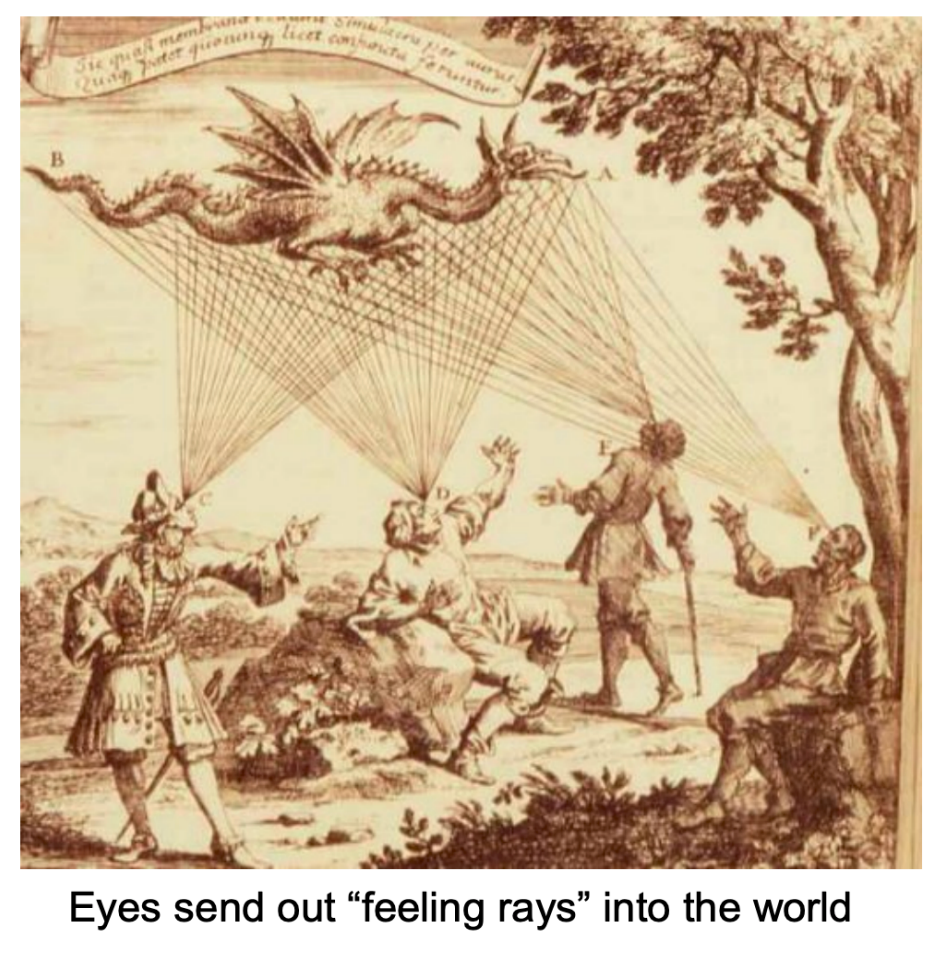
Historically people believed the eye emitted “feeler rays” into the world. In reality light leaves the source, bounces and refracts a few times, and eventually reaches the eye. Because light paths are reversible, we can trace backwards from the eye (camera) to the light source.
3 Ray Casting
Ray casting was introduced by Appel in 1968 and is the most basic form of ray tracing:
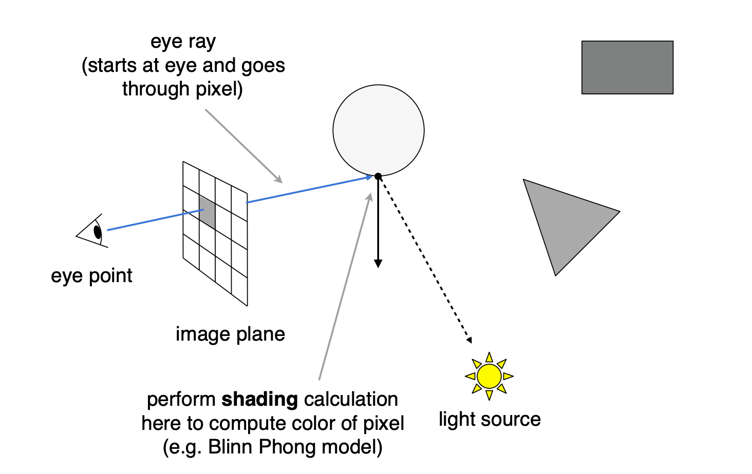
- For each pixel, shoot one ray from the camera (primary ray / eye ray)
- Find the closest intersection between the ray and the scene
- From that point, shoot a shadow ray toward each light to test occlusion
- Compute the pixel colour from the local shading at the hit point (local lighting only — no reflection or refraction)
Ray Casting in the Pinhole Camera Model
camera (eye) → pixel → scene intersection → light source
- Shoot one ray from the camera through the centre of each pixel
- Find the closest intersection with the scene
- Shoot a shadow ray from that point toward the light to test occlusion
- Compute local shading (e.g. the Blinn-Phong model)
Limitation: only direct lighting is computed — no reflection, no refraction (rays can reflect many times, recursively).
4 Whitted-Style Ray Tracing
Core Idea
Whitted proposed recursive ray tracing in 1980 (“An improved illumination model for shaded display”), extending ray casting with recursive tracing of reflected and refracted rays.
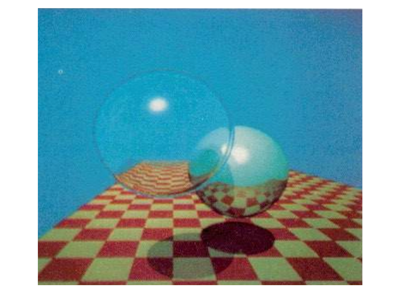
How render times evolved: Whitted’s classic 1979 image “Spheres and Checkerboard” took roughly 74 minutes on a VAX 11/780 (1979), about 6 seconds on a PC (2006), and about 1/30 of a second on a GPU (2012).
Algorithm
- Shoot a primary ray from the camera through the pixel
- Find the closest intersection
- Compute direct lighting at the hit point (shadow rays toward the lights)
- If the surface is specular, recursively shoot a reflected ray
- If the surface is transparent / refractive, recursively shoot a refracted ray
- Final colour = direct lighting + reflection contribution + refraction contribution
Ray Terminology
| Term | Meaning |
|---|---|
| Primary ray | The ray from the camera through the pixel into the scene |
| Secondary rays | Reflected rays (specular reflection) and refracted rays (specular transmission) generated recursively at hit points |
| Shadow rays | Rays from the shading point toward the light, used for occlusion tests |
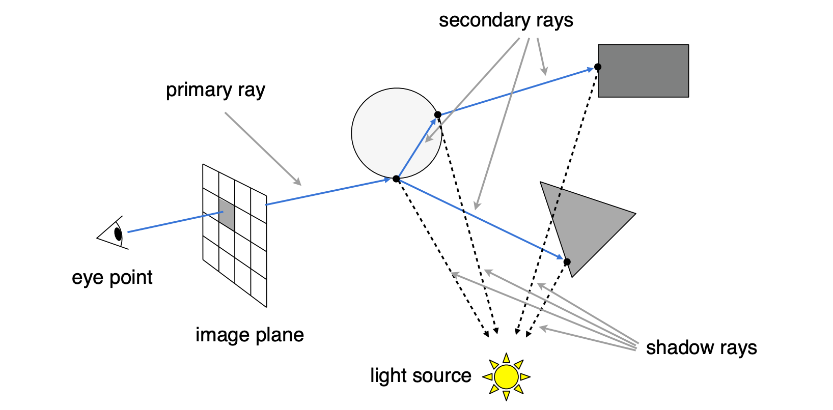
Pseudocode
trace(ray, depth):
    if depth > MAX_DEPTH:
        return BLACK

    hit = find_nearest_intersection(ray, scene)
    if not hit:
        return BACKGROUND_COLOR

    color = shade(hit)  // direct lighting

    if hit.material is reflective:
        reflect_ray = reflect(ray, hit.normal)
        color += kr * trace(reflect_ray, depth + 1)

    if hit.material is transparent:
        refract_ray = refract(ray, hit.normal, ior)
        color += kt * trace(refract_ray, depth + 1)

    return color
Problems with Whitted-Style Ray Tracing
- Specular materials: always performs perfect specular reflection/refraction, which is wrong for glossy materials
- Diffuse surfaces: rays stop bouncing at diffuse surfaces, losing indirect lighting between diffuse surfaces
- Not physically correct: cannot produce effects such as colour bleeding
These problems are solved later by path tracing.
5 Ray–Surface Intersection
Ray Equation
A ray is defined by an origin $\vec{o}$ and a (normalised) direction $\vec{d}$:
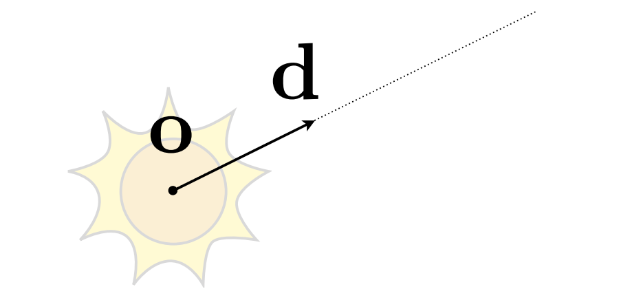
Here $t$ is the parameter along the ray (a “time”).
Ray–Sphere Intersection
Sphere equation (centre $\vec{c}$, radius $R$): a point $\vec{p}$ on the sphere is at distance $R$ from the centre:
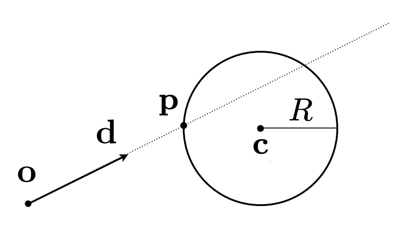
A point lying on both the ray and the sphere satisfies both equations. Substitute the ray equation into the sphere equation:
$$ (\vec{o} + t\vec{d} - \vec{c})^2 - R^2 = 0 $$Expanding gives a quadratic in $t$, namely $at^2 + bt + c = 0$:
$$ a = \vec{d} \cdot \vec{d} $$$$ b = 2(\vec{o} - \vec{c}) \cdot \vec{d} $$$$ c = (\vec{o} - \vec{c}) \cdot (\vec{o} - \vec{c}) - R^2 $$Solve:
$$ t = \frac{-b \pm \sqrt{b^2 - 4ac}}{2a} $$- Take the smallest positive real root $t$ as the intersection
- If the discriminant $b^2 - 4ac < 0$, the ray misses the sphere
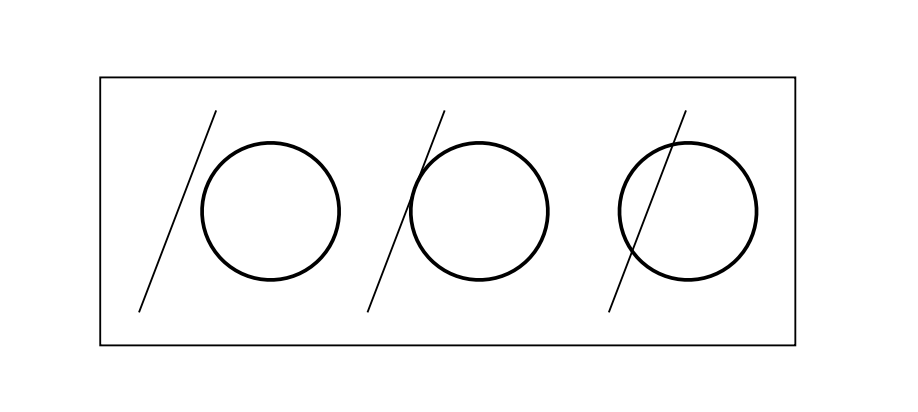
Ray–Implicit Surface Intersection
General implicit surface: $\vec{p} : f(\vec{p}) = 0$
Substitute the ray equation: $f(\vec{o} + t\vec{d}) = 0$
Solve for real, positive roots.
Ray–Plane Intersection
A plane is defined by a normal $\vec{N}$ and a point $\vec{p}'$ on the plane: for any point $\vec{p}$ on the plane, the segment from $\vec{p}'$ to $\vec{p}$ lies in the plane and is therefore perpendicular to the normal:
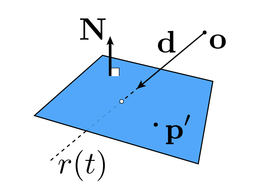
Substituting the ray equation:
$$ (\vec{o} + t\vec{d} - \vec{p}') \cdot \vec{N} = 0 $$Solving for $t$:
$$ t = \frac{(\vec{p}' - \vec{o}) \cdot \vec{N}}{\vec{d} \cdot \vec{N}} $$Then check $0 \leq t < \infty$. If $\vec{d} \cdot \vec{N} = 0$, the ray direction is perpendicular to the normal (equivalently, the ray is parallel to the plane), the denominator is zero and there is no intersection. (If the origin also lies exactly in the plane, the whole ray lies in the plane and there is still no unique intersection.)
Perpendicular vs parallel: the normal $\vec{N}$ is itself perpendicular to the plane, so “a vector perpendicular to $\vec{N}$” is exactly “a vector lying in / parallel to the plane”. The plane equation $(\vec{p} - \vec{p}') \cdot \vec{N} = 0$ filters points on the plane by requiring their connecting segment to be perpendicular to the normal; $\vec{d} \cdot \vec{N} = 0$ says the ray direction is parallel to the plane and can never pierce it. Both zero dot products express the same geometric condition — only the reference object (normal vs plane) differs.
Ray–Triangle Intersection
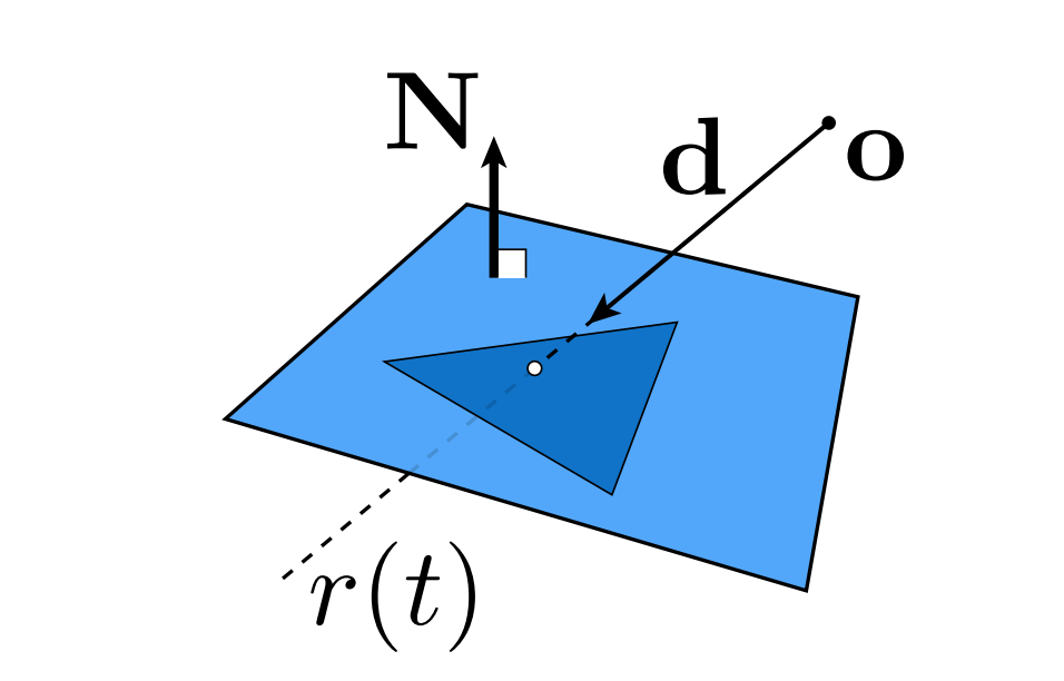
Why it matters:
- Rendering: visibility, shadows, lighting
- Geometry: inside/outside tests
Basic idea: a triangle lies in a plane, so do it in two steps:
- Intersect the ray with the triangle’s plane
- Test whether the intersection lies inside the triangle
Möller–Trumbore Algorithm
A faster way to directly test whether a ray passes through a triangle, which returns both the parameter $t$ and the barycentric coordinates $(b_1, b_2)$.
Let the triangle vertices be $\vec{P}_0, \vec{P}_1, \vec{P}_2$, the ray origin $\vec{O}$ and direction $\vec{D}$:
$$ \vec{O} + t\vec{D} = (1 - b_1 - b_2)\vec{P}_0 + b_1\vec{P}_1 + b_2\vec{P}_2 $$Define the helper quantities:
$$ \vec{E}_1 = \vec{P}_1 - \vec{P}_0, \quad \vec{E}_2 = \vec{P}_2 - \vec{P}_0 $$$$ \vec{S} = \vec{O} - \vec{P}_0, \quad \vec{S}_1 = \vec{D} \times \vec{E}_2, \quad \vec{S}_2 = \vec{S} \times \vec{E}_1 $$The solution is:
$$ \begin{pmatrix} t \\ b_1 \\ b_2 \end{pmatrix} = \frac{1}{\vec{S}_1 \cdot \vec{E}_1} \begin{pmatrix} \vec{S}_2 \cdot \vec{E}_2 \\ \vec{S}_1 \cdot \vec{S} \\ \vec{S}_2 \cdot \vec{D} \end{pmatrix} $$Conditions:
- $t \geq 0$: the intersection lies on the ray
- $b_1 \geq 0, \; b_2 \geq 0, \; 1 - b_1 - b_2 \geq 0$: the intersection lies inside the triangle
Cost: 1 division, 27 multiplications, 17 additions (from the Möller–Trumbore paper).
6 Acceleration Structures for Ray Tracing
The Performance Problem
Naive approach: for every ray, test every triangle and keep the closest hit.
| Scene | Triangle count |
|---|---|
| San Miguel | 10.7M |
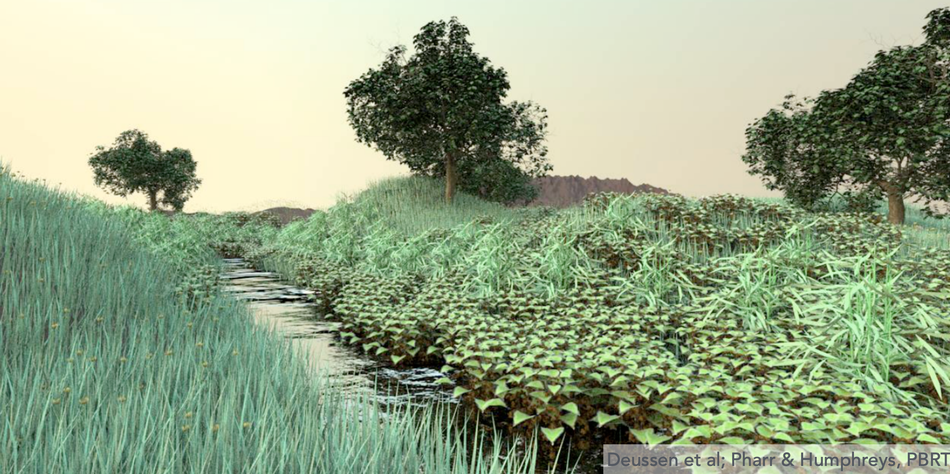
| Plant Ecosystem | 20M |
Naive complexity is roughly #pixels × #triangles × #bounces — hopelessly slow.
Bounding Volumes
Core idea: enclose complex objects with simple shapes (such as a box). If a ray misses the bounding volume, it cannot hit anything inside, so we can skip it entirely.

Axis-Aligned Bounding Box (AABB)
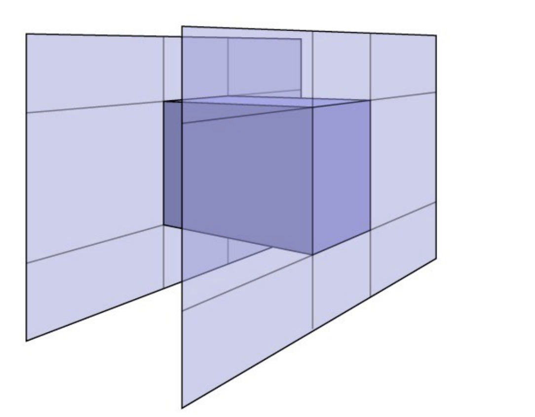
Axis-Aligned Bounding Box (AABB): every face of the box is parallel to the x, y or z axis.
Why axis-aligned: intersecting a ray with axis-aligned faces is far cheaper than with general planes.
Ray–AABB Intersection (Slab Method)
Intuition: a 3D box is the intersection of 3 pairs of parallel slabs.
2D example (3D is analogous): for each pair of slabs (one pair per axis), compute the entry and exit $t$ values:
- For each slab pair, compute $t_{min}$ and $t_{max}$
- Entry time of the 3D box: $t_{enter} = \max\{t_{min}\}$ (the largest of all $t_{min}$)
- Exit time of the 3D box: $t_{exit} = \min\{t_{max}\}$ (the smallest of all $t_{max}$)
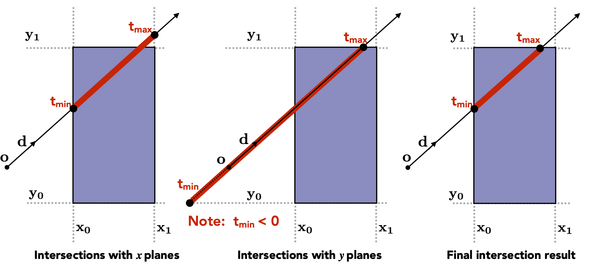
Key rules:
- The ray only enters the box after entering all slab pairs
- The ray leaves the box as soon as it leaves any slab pair
- If $t_{enter} < t_{exit}$, the ray spent some time inside the box, i.e. there is an intersection
Extra checks (a ray is not an infinite line, so the signs of $t$ matter):
| Case | Condition | Conclusion |
|---|---|---|
| $t_{exit} < 0$ | The box is behind the ray | No intersection |
| $t_{exit} \geq 0$ and $t_{enter} < 0$ | The ray origin is inside the box | Intersection |
| General case | $t_{enter} < t_{exit}$ and $t_{exit} \geq 0$ | Intersection |
Summary: a ray intersects an AABB iff
$$ t_{enter} < t_{exit} \quad \text{and} \quad t_{exit} \geq 0 $$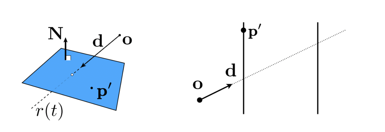
| Type | Formula |
|---|---|
| General plane | $t = \frac{(\vec{p}' - \vec{o}) \cdot \vec{N}}{\vec{d} \cdot \vec{N}}$ |
| Axis-aligned face | $t = \frac{p_x' - o_x}{d_x}$ |
7 Spatial Partitioning vs Object Partitioning
The previous section answered “how does a ray intersect a single bounding box”. This section answers: how do we use bounding boxes to speed up ray intersection against the whole scene? There are two families of answers — partition space, or partition objects.
Uniform Grids
Construction:
- Compute the scene bounding box
- Subdivide it into a uniform grid
- Store each object in the cells it overlaps
Ray traversal:
- Walk the cells in the order the ray passes through them (this is the 3D DDA algorithm)
- Test intersection against the objects in each cell
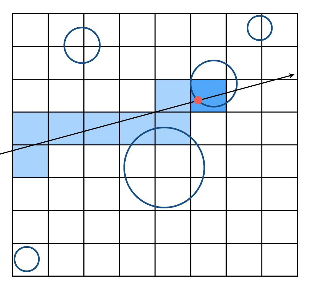
The two extremes of grid resolution:
- Too few cells (extreme: the whole scene in one cell) → every ray still tests every object, no speedup at all
- Too many cells → time is wasted traversing the grid itself
Hence a heuristic:
$$ \#\text{cells} = C \times \#\text{objs}, \quad C \approx 27 \text{ (3D)} $$When it works and when it does not:
| Scene | Result | Notes |
|---|---|---|
| Objects of similar size, evenly distributed | Good | The grid skips empty regions effectively |
| The “teapot in a stadium” problem | Bad | Very uneven distribution leaves most cells empty |
Spatial Partitioning
Divide space into non-overlapping regions. Common approaches:
| Method | Description |
|---|---|
| KD-Tree | Recursively split space with planes alternating along x/y/z |
| Oct-Tree | Recursively split space into 8 sub-cubes (3D) / 4 sub-squares (2D) |
| BSP-Tree | Recursively split space with arbitrary planes (not restricted to axis alignment) |
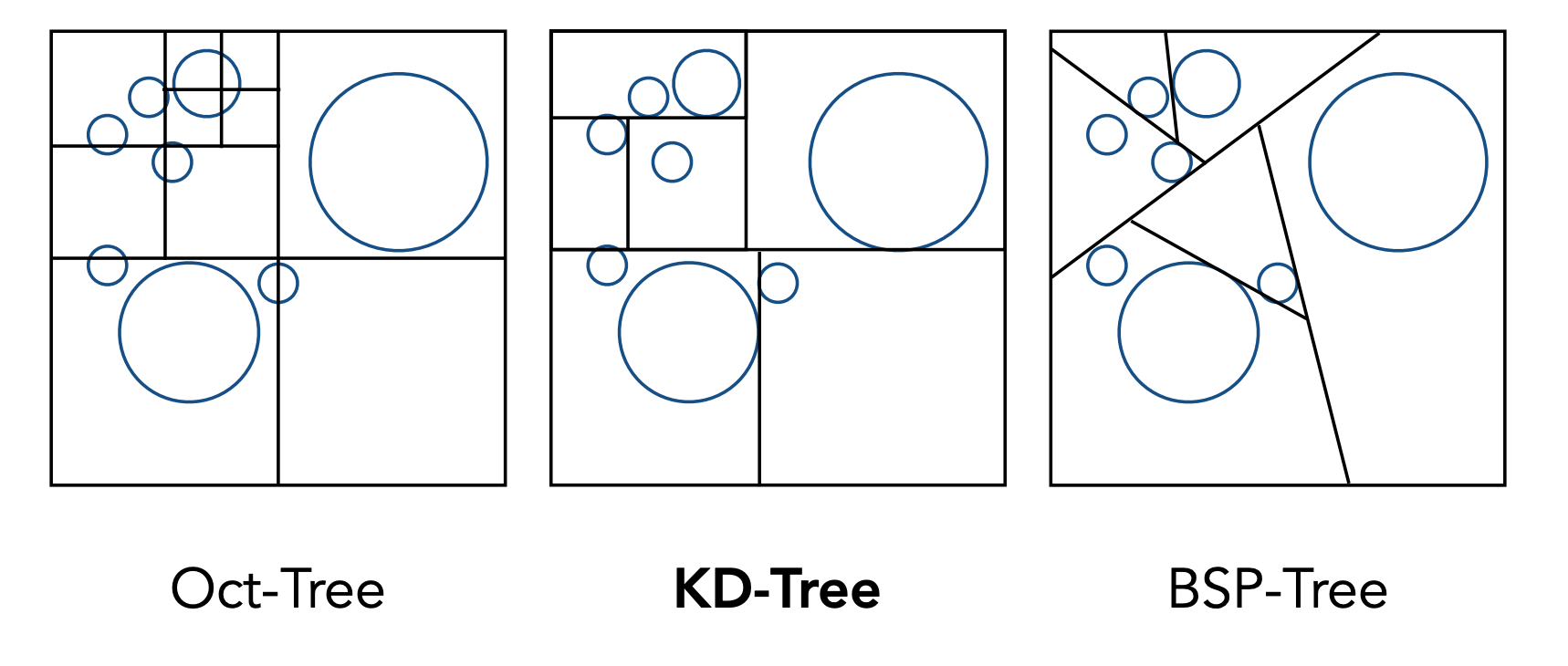
KD-Tree
Data structure:
- Internal nodes store: split axis (x/y/z), split position, child pointers (no objects)
- Leaf nodes store: the object list
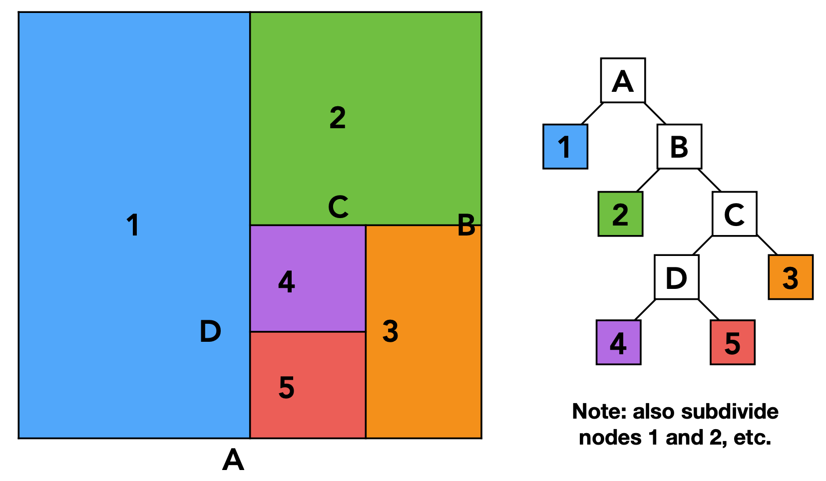
Traversal:
- Start at the root and test whether the ray intersects the node’s bounding box
- For an internal node, use the splitting plane to choose the traversal order (near child first)
- For a leaf node, test intersection against all its objects
- Return the closest hit
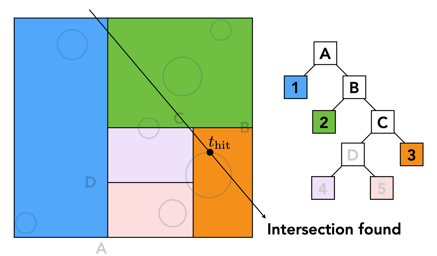
As shown above, we walk the binary tree checking for ray intersections, descending from parent to child.
Problems with KD-Tree:
- An object may span several regions and end up stored in multiple leaves
- Triangle–bounding-box intersection tests are complicated
Object Partitioning: BVH (Bounding Volume Hierarchy)
Core idea: recursively split the set of objects into two groups and compute a bounding box for each. Unlike spatial partitioning, BVH partitions objects, not space.
- Find a bounding box
- Recursively split the objects inside into two parts
- Recompute the two resulting bounding boxes
- Stop when a box contains few enough objects
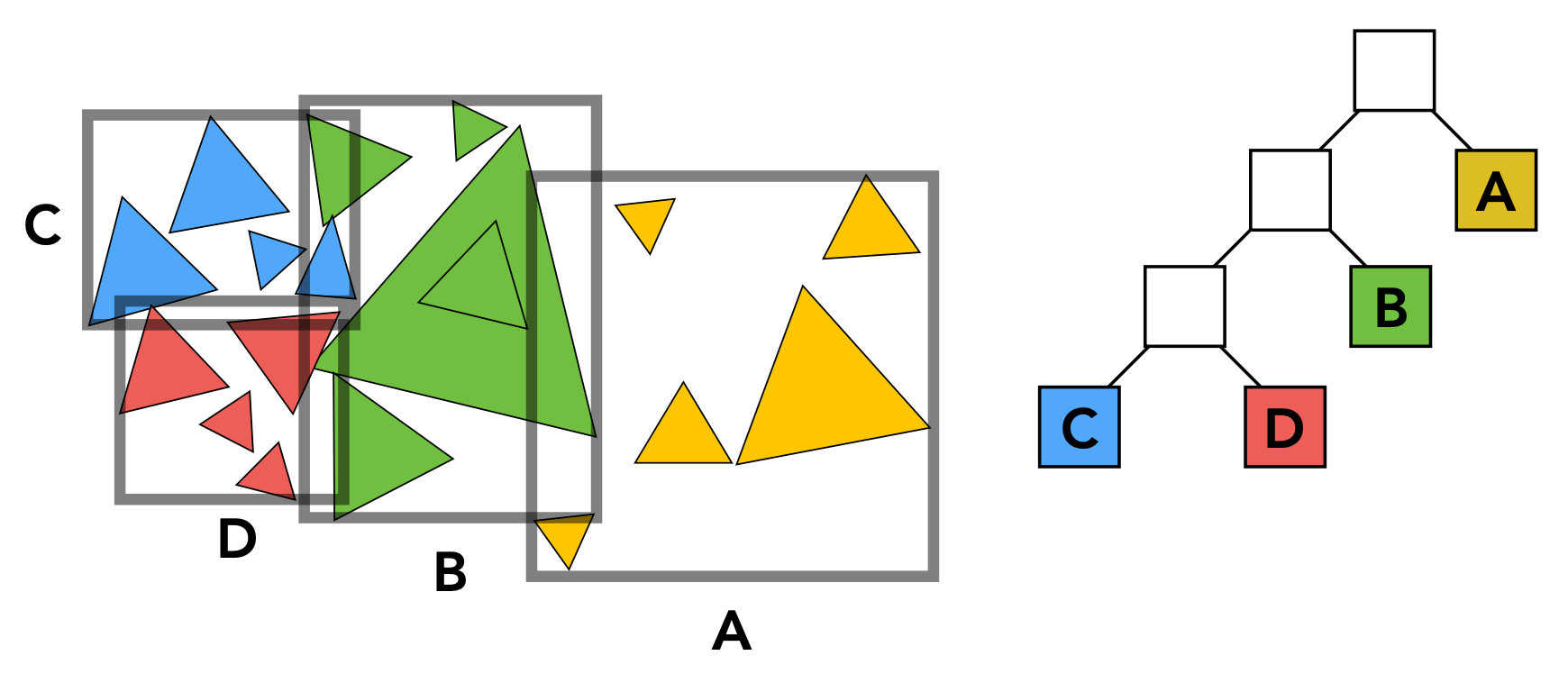
BVH Construction
How to split:
- Always split along the longest axis of the node
- Split at the median object position (keeps the two subtrees balanced), which can be done efficiently with quickselect
Quickselect: pick a pivot, partition the array into “less than or equal to pivot” and “greater than pivot” with one pass so the pivot lands in its final position, then recurse on the left and right sides until you reach the median.
Termination:
- Stop when a node contains few enough objects (e.g. 5)
BVH Data Structure
- Internal nodes store: bounding box, child pointers
- Leaf nodes store: bounding box, object list
- Every node represents a subset of the scene’s objects
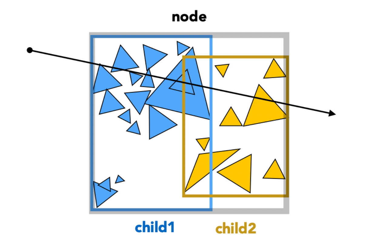
BVH Traversal
Intersect(Ray ray, BVH node) {
    if (ray misses node.bbox) return;

    if (node is leaf node)
        test intersection with all objs;
        return closest intersection;

    hit1 = Intersect(ray, node.child1);
    hit2 = Intersect(ray, node.child2);
    return the closer of hit1, hit2;
}
Spatial vs Object Partitioning
| Property | Spatial partitioning (KD-Tree) | Object partitioning (BVH) |
|---|---|---|
| What is partitioned | Space | The set of objects |
| Region overlap | Non-overlapping | Bounding boxes may overlap |
| Object membership | One object may appear in several regions | Each object belongs to exactly one subset |
| Best for | Static scenes | Dynamic scenes (rebuild locally) |
| Practical use | Rare | Most common |
BVH is by far the most widely used acceleration structure in ray tracing.
8 Radiometry
Motivation
In the Blinn-Phong model the light intensity $I$ is just a number (say 10) — but “10 what?” has no clear physical meaning. Radiometry provides a physically correct system of light measurement.
Radiometry is the system and set of methods for measuring light, able to quantify the spatial properties of light precisely. When learning a new subject it helps to walk through three questions: why learn it, what it is, and only then how to learn it.
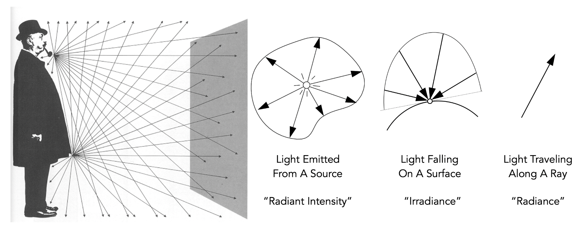
Basic Quantities
| Quantity | Symbol | Definition | Unit |
|---|---|---|---|
| Radiant energy | $Q$ | Energy of electromagnetic radiation | Joule (J) |
| Radiant flux / power | $\Phi$ | Radiant energy per unit time, $\Phi = \frac{dQ}{dt}$ | Watt (W) or lumen (lm) |
| Radiant intensity | $I(\omega)$ | Power per unit solid angle, $I = \frac{d\Phi}{d\omega}$ | W/sr or cd (candela) |
| Irradiance | $E(x)$ | Power per unit area, $E = \frac{d\Phi}{dA}$ | $W/m^2$ or lux |
| Radiance | $L(p, \omega)$ | Power per unit solid angle per unit projected area | $W/(sr \cdot m^2)$ or nit |
Solid Angle
Angle: ratio of arc length to radius, $\theta = \frac{l}{r}$; a full circle is $2\pi$ radians.
Solid angle: ratio of spherical surface area to radius squared:
$$ \Omega = \frac{A}{r^2} $$A full sphere spans $4\pi$ steradians (sr).
Differential solid angle: an infinitesimal solid angle, describing the “angular extent” around a direction in 3D space.
$$ dA = (r \, d\theta)(r \sin\theta \, d\phi) = r^2 \sin\theta \, d\theta \, d\phi $$$$ d\omega = \frac{dA}{r^2} = \sin\theta \, d\theta \, d\phi $$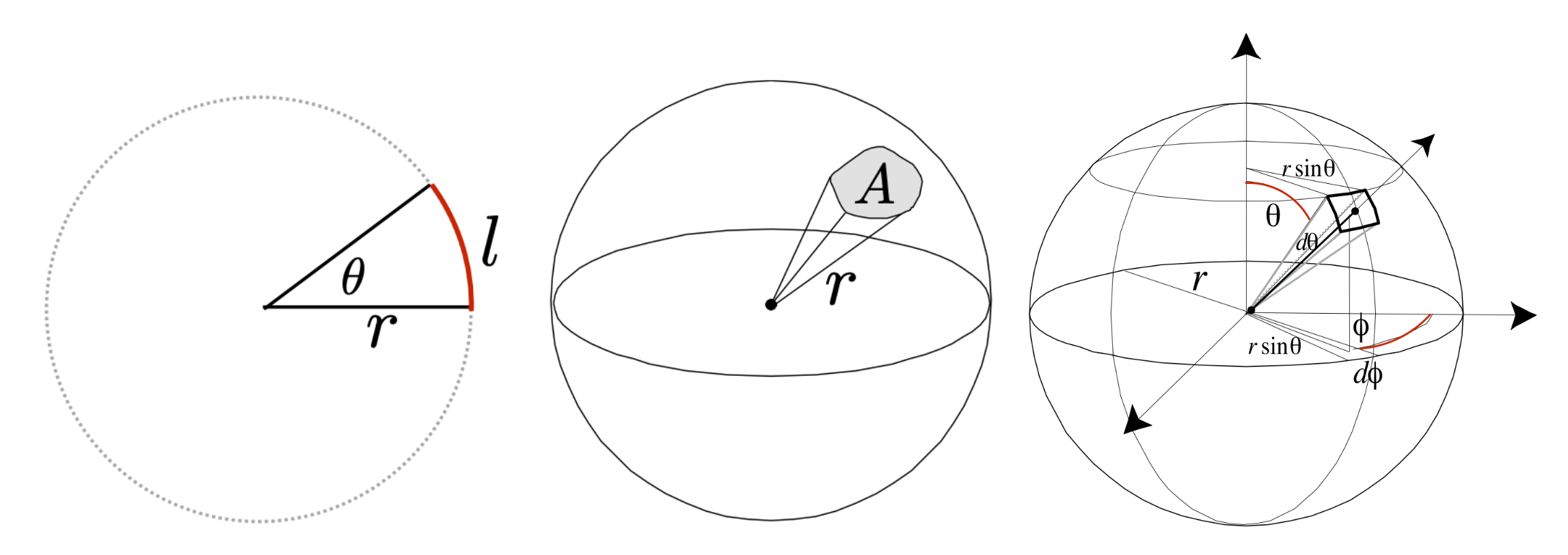
Verification: solid angle of a full sphere:
$$ \Omega = \int_{S^2} d\omega = \int_0^{\pi} \int_0^{2\pi} \sin\theta \, d\phi \, d\theta = 2\pi \left[ -\cos\theta \right]_0^{\pi} = 4\pi $$Radiant Intensity
$$ I(\omega) = \frac{d\Phi}{d\omega} $$Isotropic point light source:
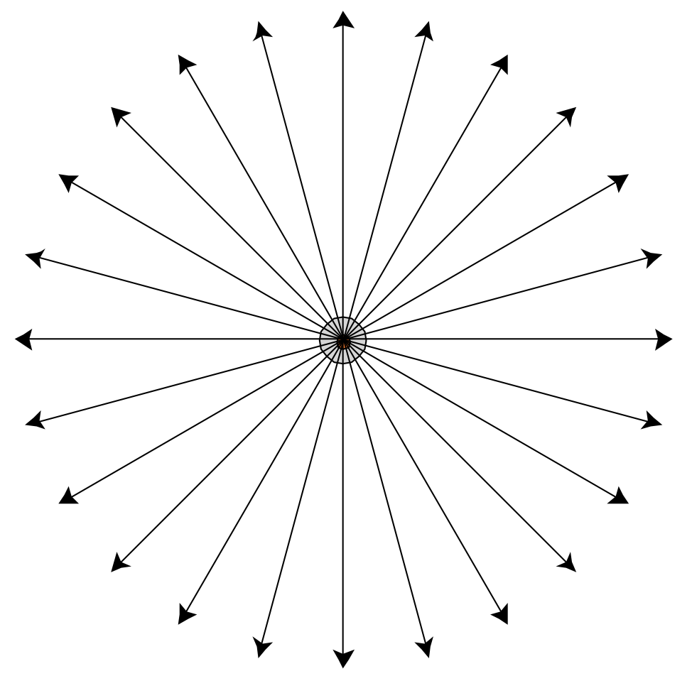
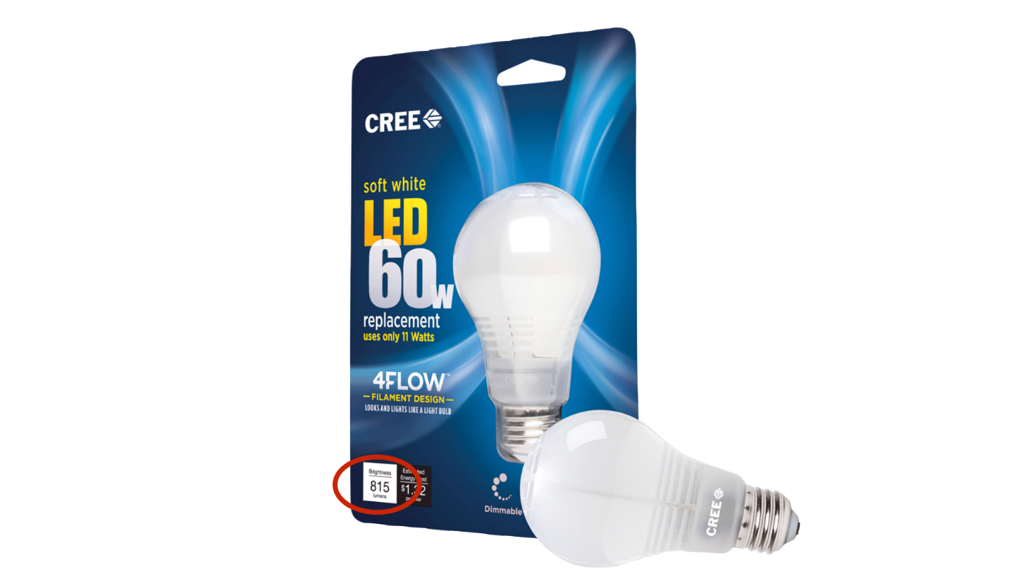
Example: an isotropic 815 lumen LED lamp → radiant intensity $= 815 / (4\pi) \approx 65$ candela.
Note: the candela is one of the seven base units of the International System of Units (SI).
Irradiance
Irradiance describes the radiant power incident on a unit area of a surface. $E$ denotes irradiance, $\Phi$ is radiant energy per unit time, and $A$ is the receiving area.
Physical meaning: radiant energy received per unit time per unit area.
$$ E(x) = \frac{d\Phi(x)}{dA} $$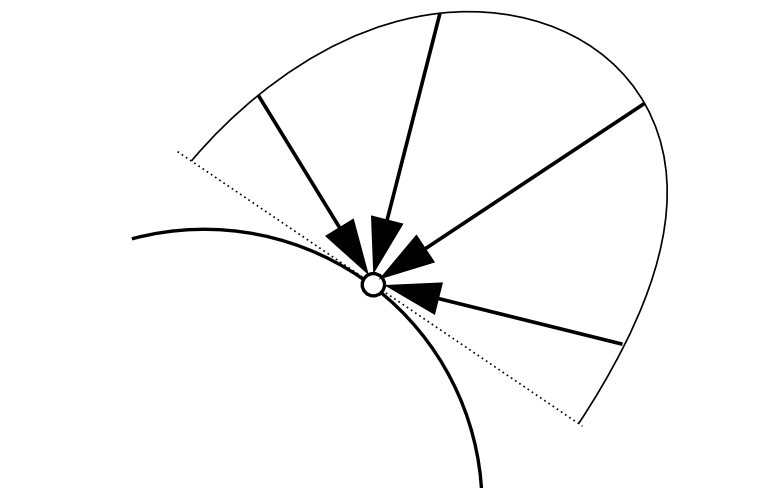
Lambert’s cosine law: irradiance is proportional to the cosine of the angle between the light direction and the surface normal.
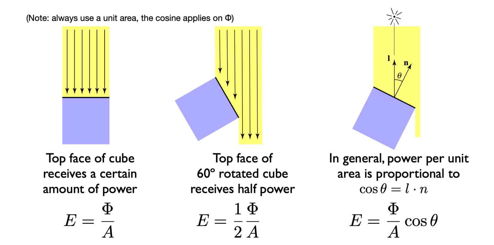
Cube example: the top face of the cube receives $E = \Phi/A$; after rotating the cube by 60°, the received power is halved, $E = \Phi/2A$. In general, power per unit area is proportional to $\cos\theta = l \cdot n$.
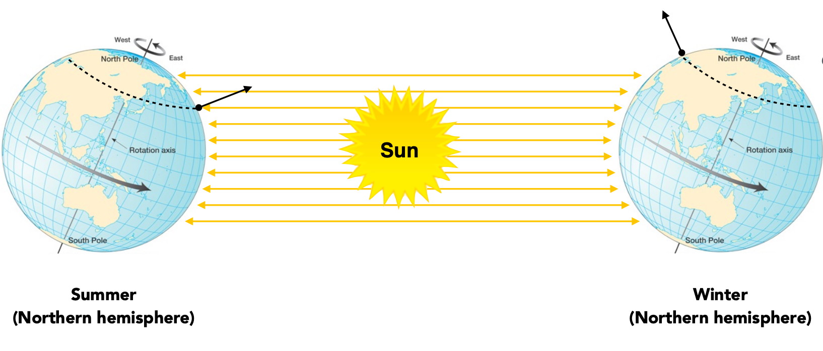
Application: the seasons. Earth’s axis is tilted by about 23.5°, so the incidence angle of sunlight varies and irradiance follows the cosine.
Irradiance falloff: how irradiance weakens with distance, angle and medium. For a point light source, irradiance at distance $r$ is inversely proportional to $r^2$:
Starting at radius 1 where $E = \frac{\Phi}{4\pi}$, after the light spreads out to radius $r$ the irradiance becomes:
$$ E' = \frac{\Phi}{4\pi r^2} = \frac{E}{r^2} $$Radiance
Radiance is the most central quantity in radiometry: radiant power per unit projected area per unit solid angle. It is the foundation of the rendering equation and the “universal currency” for describing light transport in computer graphics.
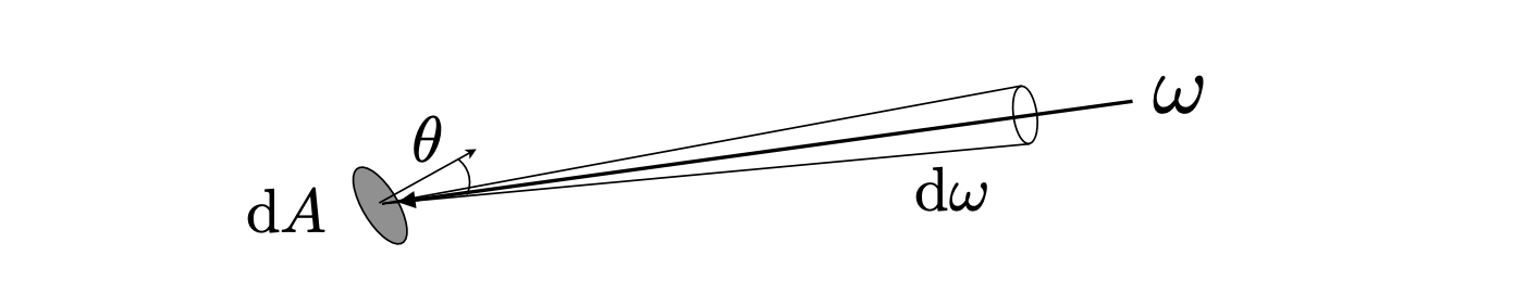
where $\cos\theta$ accounts for the projected area.
Relationships with other quantities:
| Relationship | Expression |
|---|---|
| Radiance = irradiance / solid angle | $L(p, \omega) = \frac{dE(p)}{d\omega \cos\theta}$ |
| Radiance = intensity / projected area | $L(p, \omega) = \frac{dI(p, \omega)}{dA \cos\theta}$ |
Incident radiance: irradiance arriving at a surface per unit solid angle.
Exiting radiance: radiant intensity leaving a surface per unit projected area.
Irradiance and Radiance
Irradiance is the total power received by an area $dA$; radiance is the power received by $dA$ from a direction $d\omega$.
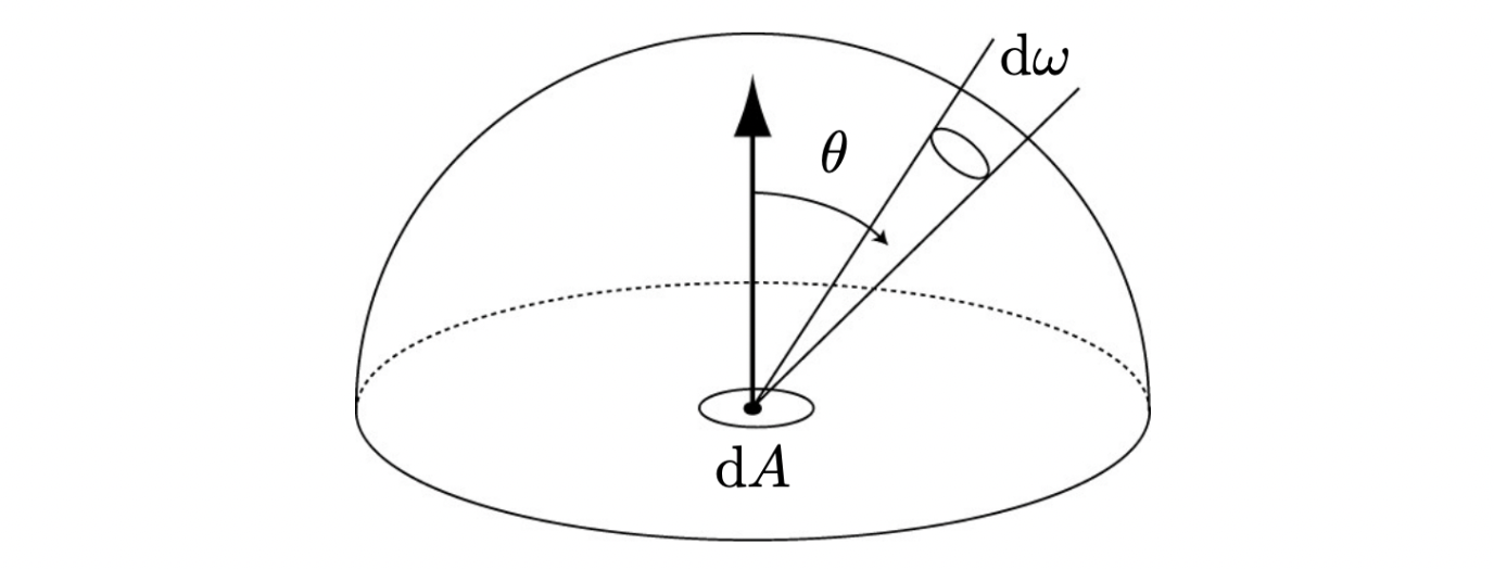
where $H^2$ is the unit hemisphere and $\cos\theta$ is the angle between the incident direction and the normal.
$$ dE(p, \omega) = L_i(p, \omega) \cos\theta \, d\omega $$$$ E(p) = \int_{H^2} L_i(p, \omega) \cos\theta \, d\omega $$Differential relation (point level): of the radiance $L_i$ coming from the infinitesimal solid angle $d\omega$, only its component perpendicular to the surface (multiplied by $\cos\theta$) contributes to irradiance.
Integral relation (surface level): total irradiance is the solid-angle integral of the incoming radiance from all directions, cosine-weighted.
| Scene | Radiance $L$ | Irradiance $E$ |
|---|---|---|
| A single laser beam | High (direction concentrated) | Low (covers a tiny solid angle) |
| Uniform ambient light | Low (spread over all directions) | High (accumulates all directions) |
| Facing the sun | Sun-direction $L$ is very high | High ($\cos\theta \approx 1$) |
| At an angle to the sun | Sun-direction $L$ unchanged | Low ($\cos\theta < 1$) |
Calculus Foundations: Differentiation and Integration
Differentiation is the art of “splitting the whole into parts”; integration is the science of “gathering the parts into a whole”. Through the fundamental theorem of calculus they mirror each other, together forming the language that describes a continuously changing world.
Differentiation — a magnifying glass on change
Essence: linearise complex change, approximating a curve with its tangent.
| Viewpoint | Description |
|---|---|
| Geometric | Replace the curve’s trend with the tangent slope |
| Physical | Instantaneous velocity, acceleration, density |
| Algebraic | $dy = f'(x)dx$, the leading linear approximation |
What it answers: given the whole / position, find the rate of change / instantaneous state.
| Question | Real-world scene | Answer from differentiation |
|---|---|---|
| How fast? | Car speedometer | Derivative of position: $v = \frac{dx}{dt}$ |
| Which trend? | Is the stock rising or falling? | Slope of the price curve |
| When optimal? | Output that maximises profit | Set $\frac{dP}{dQ} = 0$ |
| Local behaviour? | Tangent direction at a point | Gradient $\nabla f$ |
| Sensitivity? | Effect of a parameter change | Partial derivative $\frac{\partial y}{\partial x}$ |
Workflow in radiometry: describe the “instantaneous” behaviour of local light transport.
| Step | Operation | Radiometry example |
|---|---|---|
| 1. Identify the differential | Determine the infinitesimal | $d\omega$, $dA$, $d\Phi$ |
| 2. Build the differential relation | Write $dX = f \cdot dY$ | $d\Phi = L \cdot dA \cos\theta \cdot d\omega$ |
| 3. Differentiate | Compute the rate of change | $\nabla L$, BRDF differentials |
| 4. Interpret physically | Give it geometric meaning | Light per unit area / per unit angle |
Common differential formulas:
| Form | Physical meaning | Use case |
|---|---|---|
| $d\omega = \sin\theta \, d\theta \, d\phi$ | Differential solid angle | Direction sampling, change of variables |
| $dA_{proj} = dA \cos\theta$ | Projected area element | Lambert’s cosine law |
| $d\Phi = L \, dA \cos\theta \, d\omega$ | Differential radiant flux | Foundation of the rendering equation |
| $dE = L_i \cos\theta \, d\omega$ | Differential irradiance | Light received by a surface |
Integration — an accumulator for the total
Essence: accumulate the infinitesimal parts to reconstruct the whole.
| Viewpoint | Description |
|---|---|
| Geometric | Curved areas, volumes of revolution |
| Physical | Displacement, work, charge, probability |
| Algebraic | $\int_a^b f(x)dx$, a limit of sums |
What it answers: given the rate of change / local behaviour, find the total / accumulated quantity.
| Question | Real-world scene | Answer from integration |
|---|---|---|
| How much in total? | Total displacement under varying speed | $x = \int v(t)dt$ |
| Area / volume? | Area of an irregular plot | $A = \int f(x)dx$ |
| Cumulative effect? | Work by a varying force, total heat | $W = \int F(x)dx$ |
| Probability? | Probability of a continuous random variable | $P = \int_a^b f(x)dx$ |
| Average? | Mean of a function over an interval | $\bar{f} = \frac{1}{b-a}\int_a^b f(x)dx$ |
Workflow in radiometry: compute the “accumulated” result of global light transport.
| Step | Operation | Radiometry example |
|---|---|---|
| 1. Define the domain | Fix the integration range | Hemisphere $\Omega$, surface $A$, time $t$ |
| 2. Build the integrand | Write $f(x)$ | $L_i(\omega) \cos\theta$, $f_r \cdot L_i$ |
| 3. Choose a method | Analytic / numerical | Monte Carlo, importance sampling, spherical harmonics |
| 4. Evaluate and interpret | Get the total | Irradiance $E$, outgoing radiance $L_o$, flux $\Phi$ |
Common integral formulas:
| Form | Physical meaning | Use case |
|---|---|---|
| $E = \int_{\Omega} L_i \cos\theta \, d\omega$ | Surface irradiance | Lighting, IBL |
| $L_o = \int_{\Omega} f_r L_i \cos\theta \, d\omega$ | Outgoing radiance | The rendering equation |
| $\Phi = \int_A \int_{\Omega} L \cos\theta \, d\omega \, dA$ | Total radiant flux | Light source power |
| $I = \int_A L \cos\theta \, dA$ | Radiant intensity | Point light approximation |
Fundamental theorem of calculus:
$$ \int_a^b f'(x)dx = f(b) - f(a) $$- Differentiation decomposes: $f'(x)$ is the rate of change at each point
- Integration recomposes: accumulate those rates to get the total change
Analogy:
- Differentiation = cutting a video into frames (instantaneous states)
- Integration = playing the frames back as a video (the full process)
9 BRDF and the Reflection Equation
The Physics of Reflection
Light arrives at surface point $p$ from direction $\omega_i$:
- The incident radiance $L(\omega_i)$ produces a differential irradiance on $dA$: $dE(\omega_i) = L(\omega_i) \cos\theta_i \, d\omega_i$
- That irradiance is reflected by the surface into outgoing directions $\omega_r$
- Producing a differential outgoing radiance $dL_r(\omega_r)$
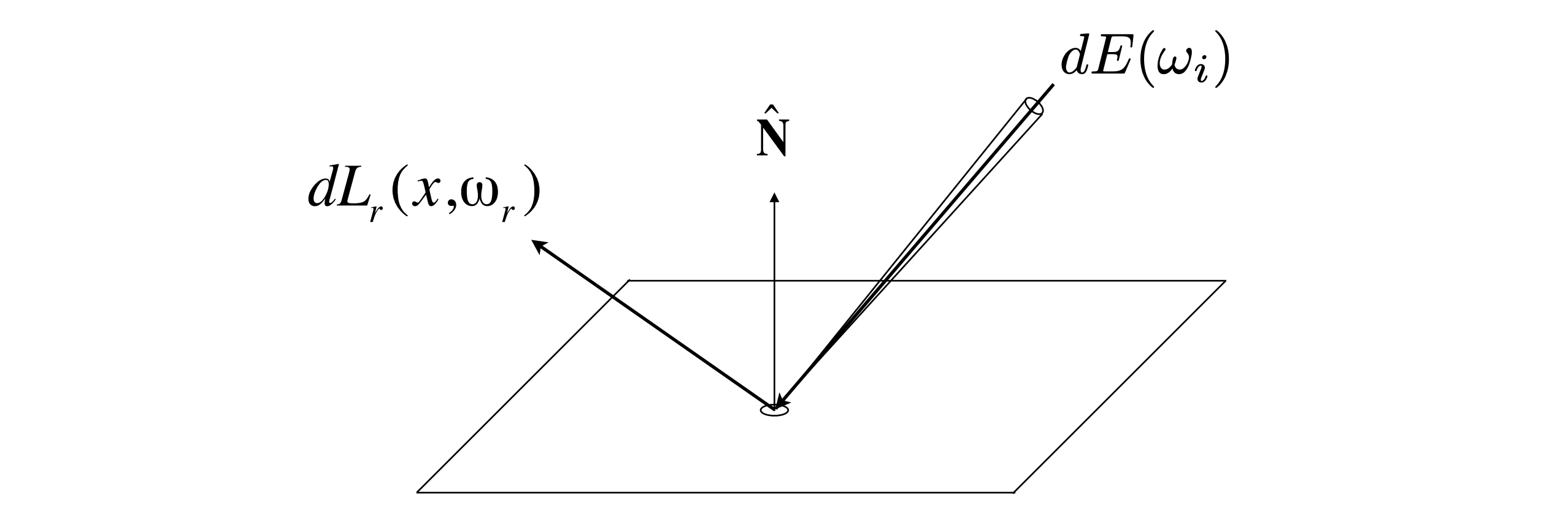
Definition of BRDF
The BRDF is the ratio of light reflected from each incident direction into each outgoing direction:
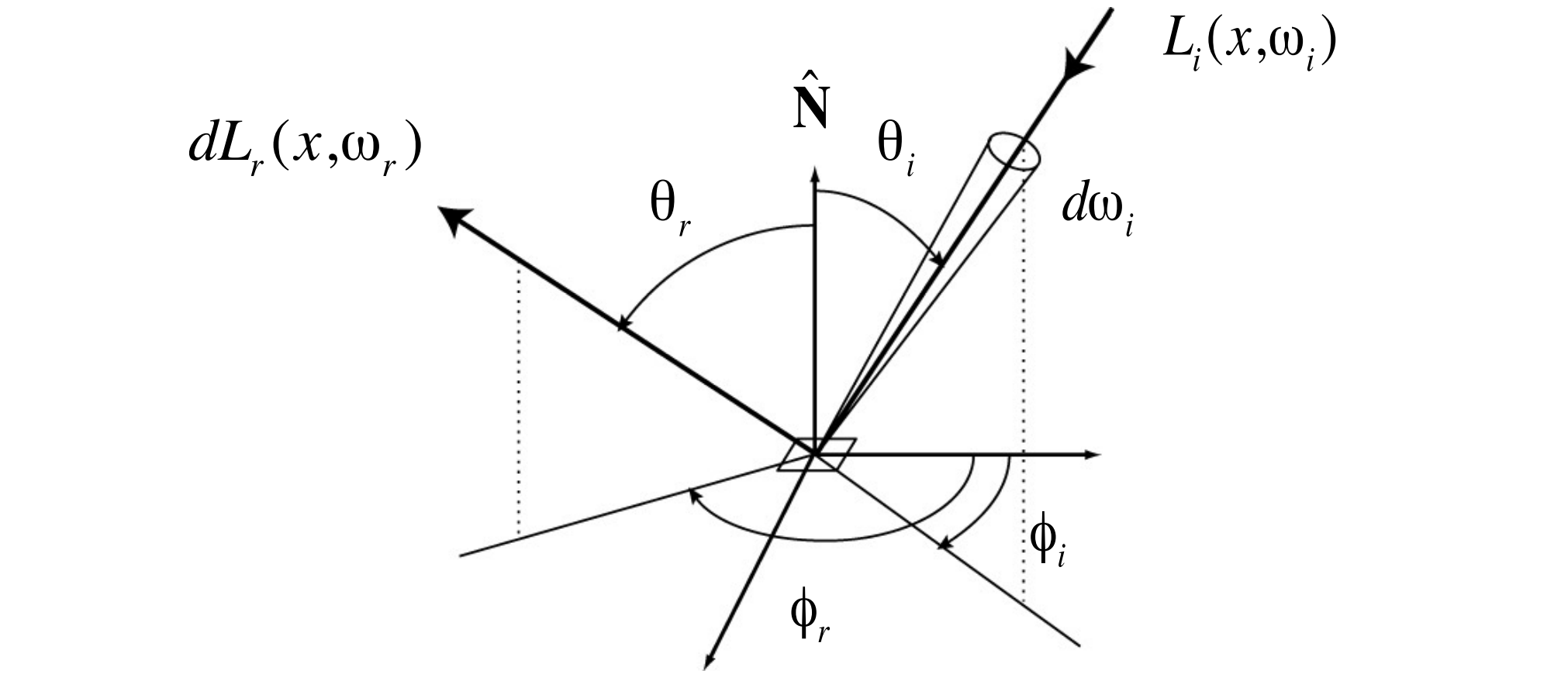
Physical meaning: the BRDF fully describes a material’s reflective behaviour — in graphics, a material is a BRDF.
The Reflection Equation
The outgoing radiance at point $p$ along $\omega_r$ is the sum (integral) over all incident directions:
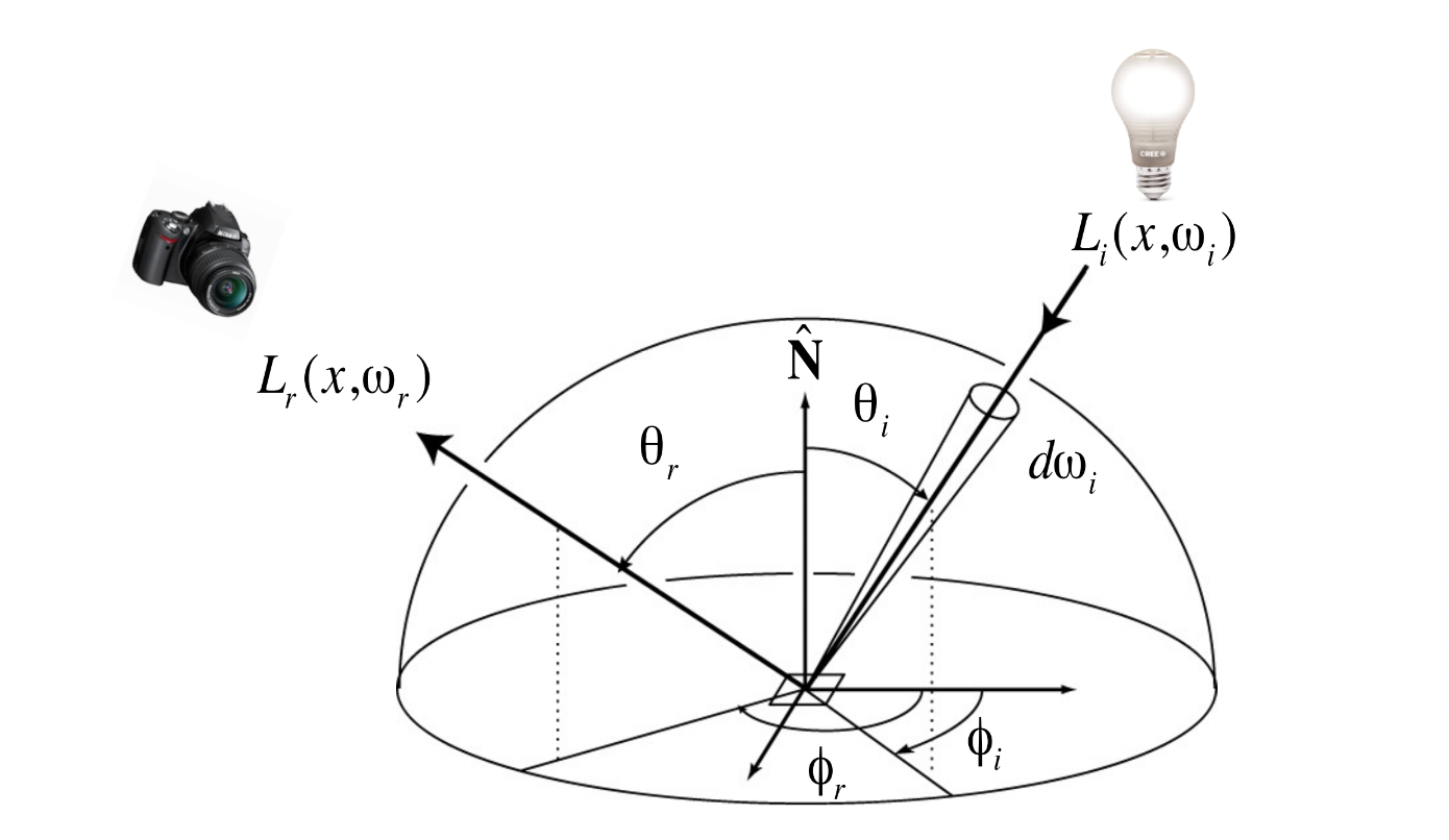
where:
- $f_r$: the BRDF (how much is reflected)
- $L_i$: incident radiance (from lights or from other objects — recursive)
- $\cos\theta_i$: cosine of the incidence angle (Lambert’s cosine law)
- $H^2$: the unit hemisphere (all incident directions)
Recursion
The reflection equation is recursive: outgoing radiance depends on incident radiance, which in turn depends on the reflected radiance of other points. That recursion is finally captured by the rendering equation.
10 The Rendering Equation
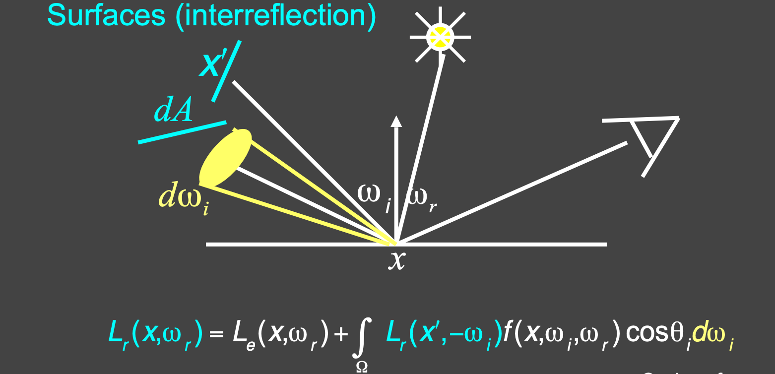
Derivation
Adding an emission term to the reflection equation gives the general form:
$$ L_o(p, \omega_o) = L_e(p, \omega_o) + \int_{\Omega^+} L_i(p, \omega_i) \, f_r(p, \omega_i, \omega_o) \, (n \cdot \omega_i) \, d\omega_i $$where:
- $L_o(p, \omega_o)$: outgoing radiance at $p$ along $\omega_o$ (unknown — this is what we solve for)
- $L_e(p, \omega_o)$: emitted radiance (known — light emitted directly by the light source)
- $L_i(p, \omega_i)$: incident radiance from direction $\omega_i$ (unknown — reflected by other points)
- $f_r(p, \omega_i, \omega_o)$: BRDF (known — determined by the material)
- $(n \cdot \omega_i) = \cos\theta_i$: cosine of the incidence angle (known)
- $\Omega^+$: the upper hemisphere (all directions pointing outward)
Note: all directions are assumed to point outward.
The rendering equation was introduced by Kajiya in 1986.
Physical Meaning
| Term | Meaning | Known/Unknown |
|---|---|---|
| $L_o(p, \omega_o)$ | Outgoing radiance (the output image) | Unknown |
| $L_e(p, \omega_o)$ | Emission | Known |
| $L_i(p, \omega_i)$ | Incident radiance (from lights or other objects) | Unknown |
| $f_r(p, \omega_i, \omega_o)$ | BRDF | Known |
| $n \cdot \omega_i$ | Cosine of the incidence angle | Known |
Mathematical View
The rendering equation is a Fredholm integral equation of the second kind, whose canonical form is:
$$ I(u) = \epsilon(u) + \int I(v) K(u, v) \, dv $$where $K(u,v)$ is the kernel.
As a linear operator:
$$ L = E + KL $$where $K$ is the light transport operator.
Series Solution
$$ L = E + KL $$$$ (I - K)L = E $$$$ L = (I - K)^{-1}E $$Expanding as a binomial series:
$$ L = (I + K + K^2 + K^3 + \cdots)E = E + KE + K^2E + K^3E + \cdots $$The physical meaning of each term:
| Term | Physical meaning | Can rasterization handle it? |
|---|---|---|
| $E$ | Light directly from the source | Yes |
| $KE$ | Direct lighting (one bounce) | Yes |
| $K^2E$ | Indirect lighting (two bounces, e.g. specular reflection) | No |
| $K^3E$ | Two rounds of indirect lighting | No |
| $K^nE$ | $n-1$ rounds of indirect lighting | No |
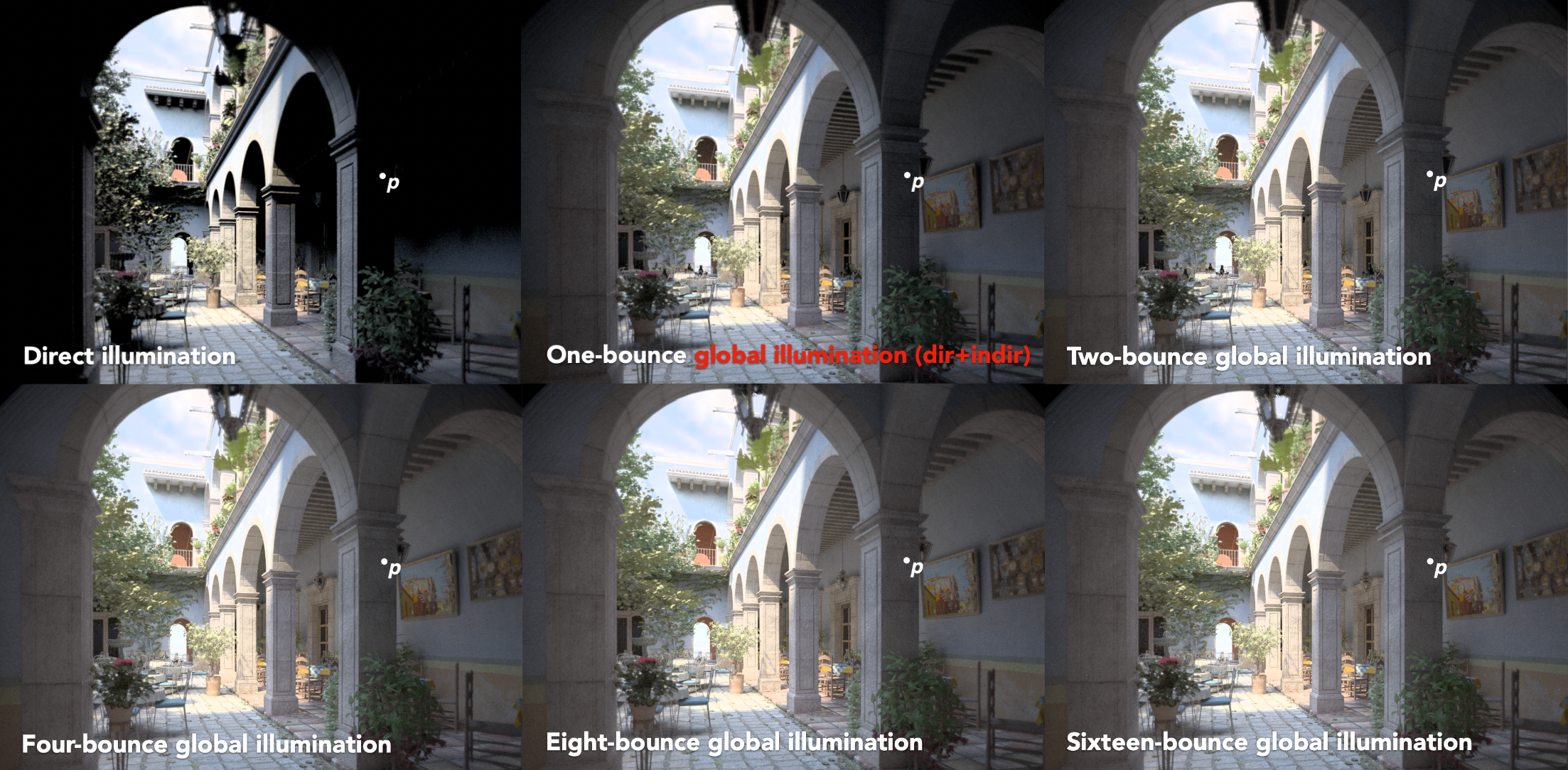
Rasterization can essentially only handle $E + KE$ (direct lighting) and cannot deal with higher-order indirect lighting. Ray tracing (path tracing) simulates all bounce orders naturally.
11 Probability and Monte Carlo Integration
Probability Review
Random variable: a quantity whose value depends on “luck”, written $X \sim p(x)$. Rolling a die: before the roll you don’t know the value; $p(x)$ describes how likely each value is.
Each face of a die is equally likely, $p_i = 1/6$. A valid distribution needs only two things: $p_i \geq 0$ and all probabilities summing to 1 (100% in total).
Expectation = average: roll the die infinitely many times — what’s the average?
$$ E[X] = \sum_{i=1}^{n} x_i p_i \qquad \xrightarrow{\text{die}} \qquad \frac{1+2+3+4+5+6}{6} = 3.5 $$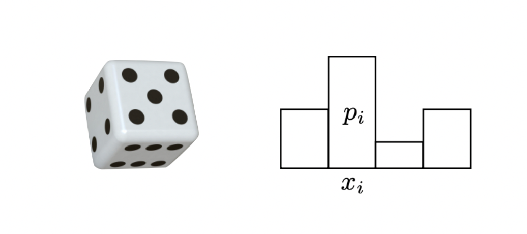
Note that 3.5 can never be rolled — the expectation is not a possible outcome but the “on average” value.
The continuous case: the value can be any number in an interval (a direction, say). The probability of any single point is 0, so probability is measured as area:
$$ P(a \leq X \leq b) = \int_a^b p(x) \, dx $$$p(x)$ is the probability density function (PDF), requiring $p(x) \geq 0$ and $\int p(x) \, dx = 1$. (A density is not a probability — it may exceed 1; the actual probability is the area under the curve.)
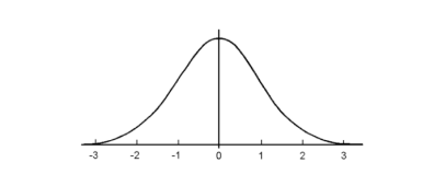
Expectation of a function of a random variable: applying a transform $Y = f(X)$ still yields a random variable, with expectation
$$ E[f(X)] = \int f(x) \, p(x) \, dx $$Intuition: draw an $X$, compute $f(X)$, and average the results weighted by how likely they are.
Monte Carlo Integration
Why we need it: the rendering equation integrates over the hemisphere, and the integrand (incident radiance $L_i$) is usually unknown and complicated. Analytic solution is infeasible, so we need a numerical method.
Definition: given a definite integral $\int_a^b f(x) \, dx$, estimate it by random sampling:
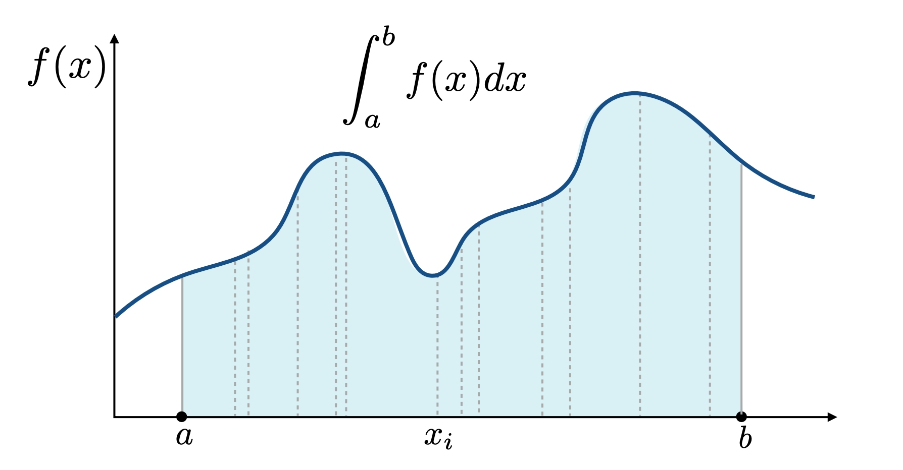
where $X_i \sim p(x)$ are random variables sampled from the PDF $p(x)$.
Unbiasedness: the Monte Carlo estimator is unbiased:
$$ E[F_N] = \int_a^b f(x) \, dx $$That is, no matter how many samples $N$ you take, the expected value of the estimate equals the true integral.
The uniform-sampling special case:
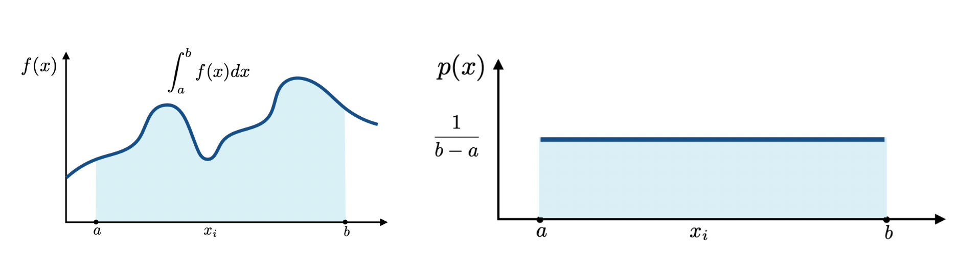
When $p(x) = \frac{1}{b-a}$ (uniform), we get
$$ F_N = \frac{b-a}{N} \sum_{i=1}^{N} f(X_i) $$Important properties:
- More samples $N$ means lower variance (a more accurate estimate)
- Sample on $x$, integrate on $x$
- Any PDF $p(x)$ works, as long as $p(x) > 0$ wherever $f(x) \neq 0$
12 Path Tracing
The Two Problems with Whitted-Style Ray Tracing
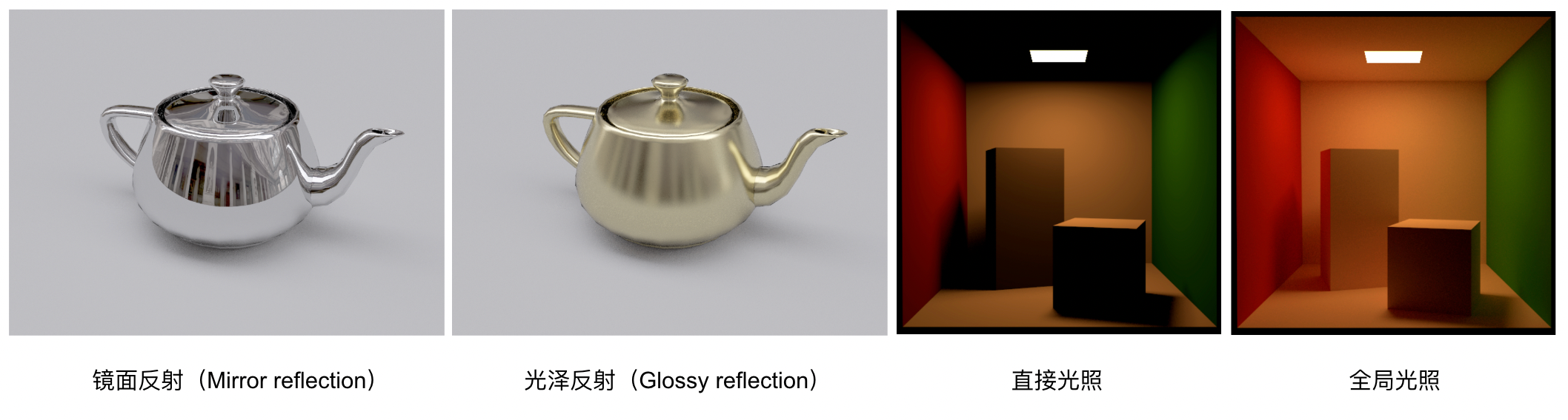
| Problem | Description |
|---|---|
| Problem 1 | Glossy materials should not perform perfect specular reflection |
| Problem 2 | Diffuse surfaces should receive indirect lighting from each other (colour bleeding) |
The rendering equation is correct, but it involves a hemisphere integral and recursion. How do we solve it numerically? Monte Carlo integration.
Monte Carlo Solution for Direct Lighting
Compute the outgoing radiance at point $p$ along $\omega_o$ (direct lighting only):
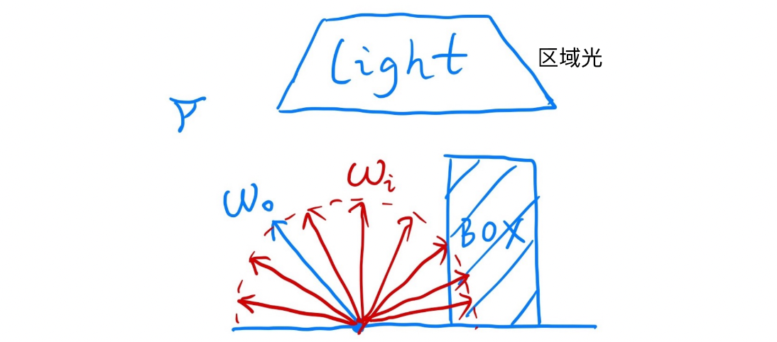
Using Monte Carlo integration with uniform sampling over the hemisphere:
$$ L_o(p, \omega_o) \approx \frac{1}{N} \sum_{i=1}^{N} \frac{L_i(p, \omega_i) \, f_r(p, \omega_i, \omega_o) \, (n \cdot \omega_i)}{p(\omega_i)} $$where $p(\omega_i) = \frac{1}{2\pi}$ is the PDF for uniform hemisphere sampling.
Pseudocode:
shade(p, wo):
    Lo = 0.0
    randomly pick N directions wi ~ pdf
    for each wi:
        shoot ray r(p, wi)
        if ray r hits the light:
            Lo += (1/N) * L_i * f_r * cos / pdf(wi)
    return Lo
Introducing Global Illumination
If the ray hits another object $q$ instead of a light, that object also reflects light back to $p$. Recurse:
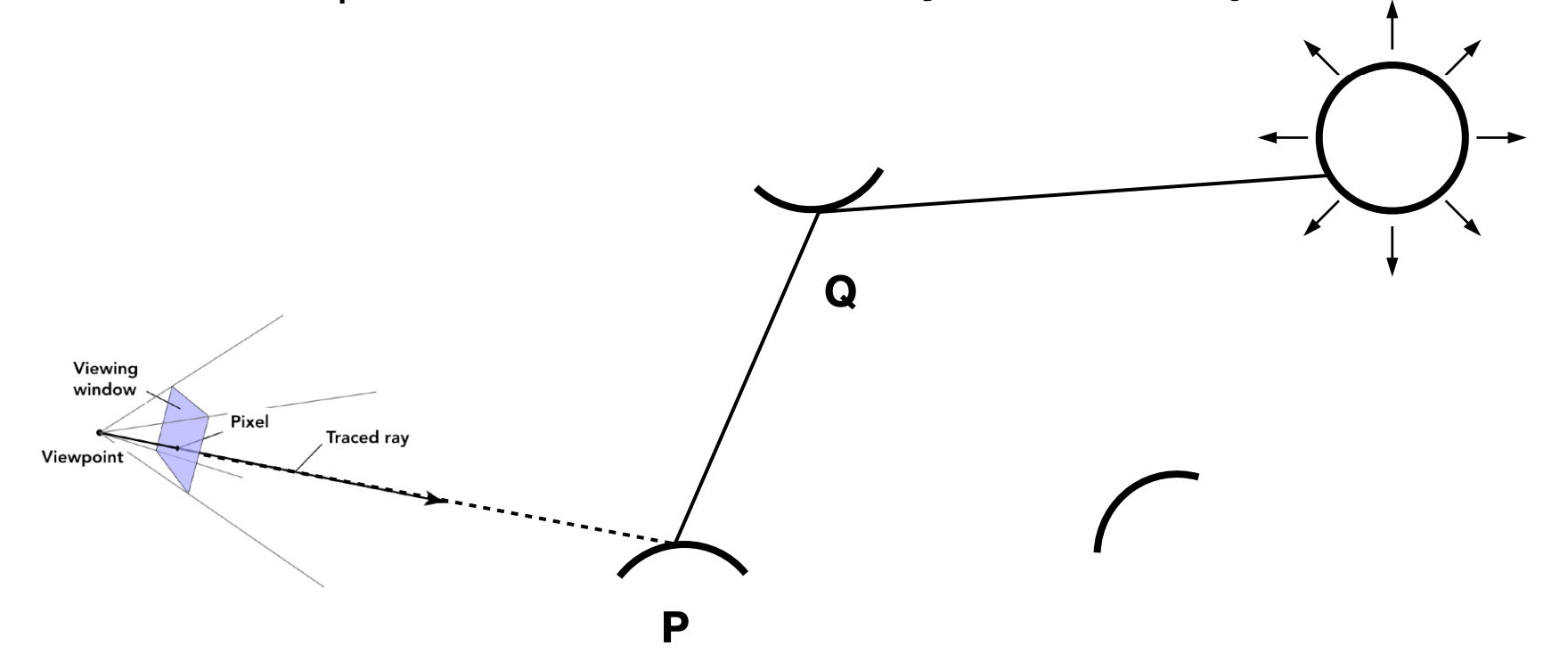
shade(p, wo):
    randomly pick N directions wi ~ pdf
    Lo = 0.0
    for each wi:
        shoot ray r(p, wi)
        if ray r hits the light:
            Lo += (1/N) * L_i * f_r * cos / pdf(wi)
        else if ray r hits object q:
            Lo += (1/N) * shade(q, -wi) * f_r * cos / pdf(wi)
    return Lo
Problem 1: Ray Explosion
Each bounce spawns $N$ rays, so after $k$ bounces there are $N^k$ rays — exponential blow-up.
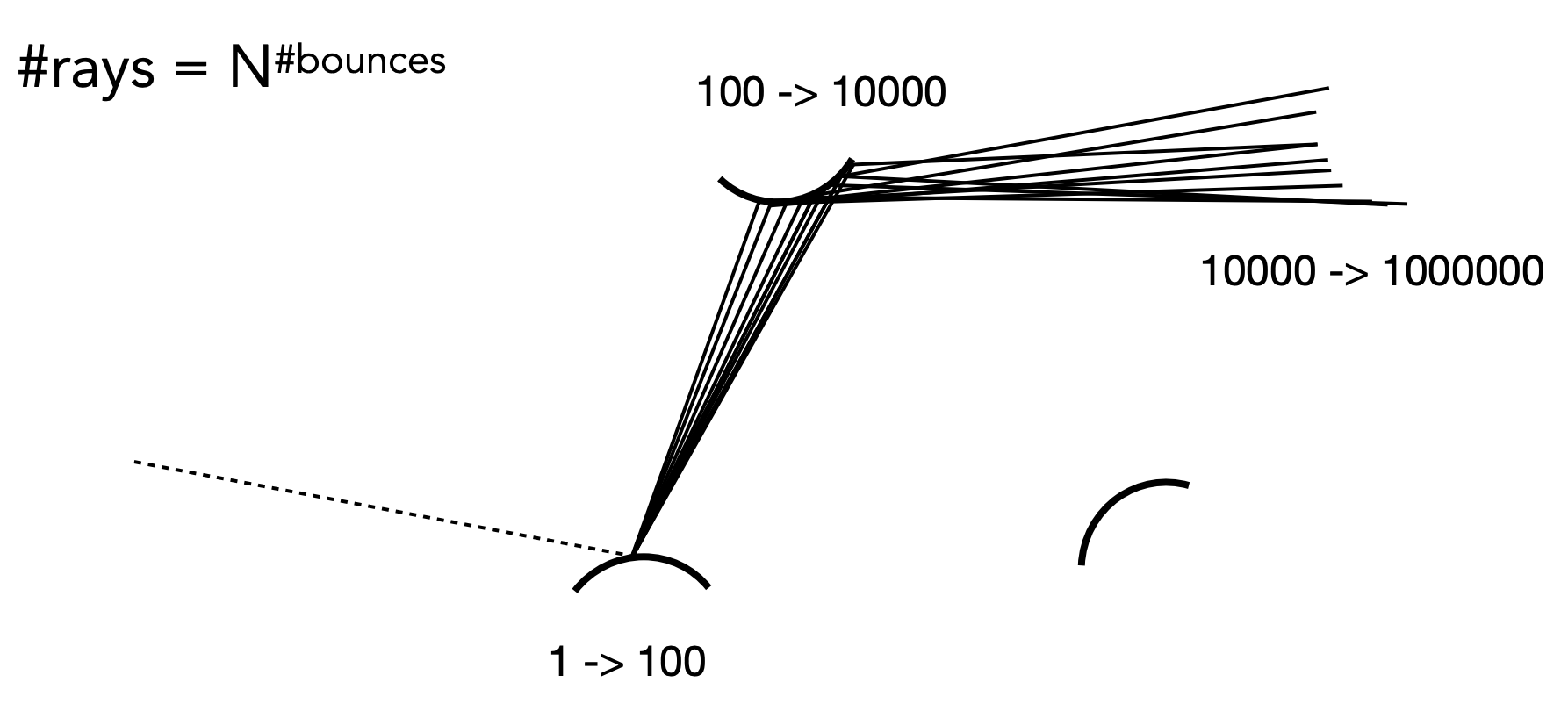
Solution: set $N = 1$ — trace exactly one ray per shading point. That is path tracing ($N \neq 1$ is called distributed ray tracing).
shade(p, wo):
    randomly pick 1 direction wi ~ pdf
    shoot ray r(p, wi)
    if ray r hits the light:
        return L_i * f_r * cos / pdf(wi)
    else if ray r hits object q:
        return shade(q, -wi) * f_r * cos / pdf(wi)
The noise problem: one path per pixel is very noisy. The fix is to shoot many paths per pixel and average.
ray_generation(camPos, pixel):
    uniformly pick N sample positions inside the pixel
    pixel_radiance = 0.0
    for each sample:
        shoot ray r(camPos, cam_to_sample)
        if ray hits scene point p:
            pixel_radiance += (1/N) * shade(p, sample_to_cam)
    return pixel_radiance
Problem 2: Recursion Never Terminates
Light bounces forever, so the recursion never stops. Truncating the bounce count loses energy.
Solution: Russian roulette (RR)
Idea:
- Choose a probability $P$ ($0 < P < 1$)
- With probability $P$: keep tracing and return the result divided by $P$, i.e. $L_o / P$
- With probability $1 - P$: stop and return 0
The expectation is unchanged:
$$ E = P \cdot \frac{L_o}{P} + (1 - P) \cdot 0 = L_o $$Pseudocode:
shade(p, wo):
    set probability P_RR
    uniformly pick ksi in [0, 1]
    if (ksi > P_RR) return 0.0

    randomly pick 1 direction wi ~ pdf
    shoot ray r(p, wi)
    if ray r hits the light:
        return L_i * f_r * cos / pdf(wi) / P_RR
    else if ray r hits object q:
        return shade(q, -wi) * f_r * cos / pdf(wi) / P_RR
Optimisation: Direct Light Sampling
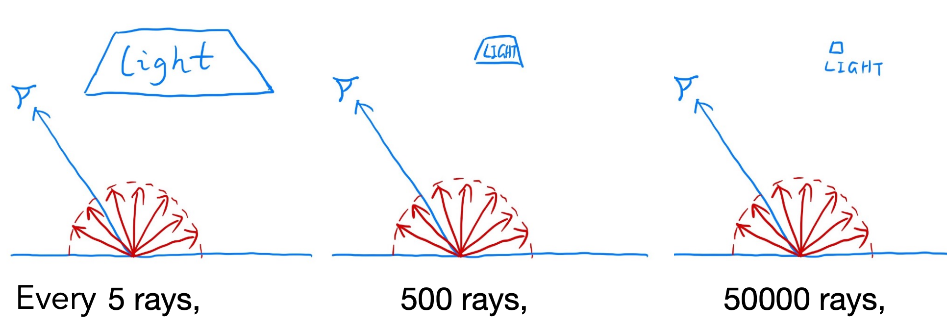
Problem: when sampling the hemisphere uniformly, most rays are “wasted” (they miss the light). Only about 1 ray in 5 hits the light.
Solution: sample the light directly.
Monte Carlo allows any sampling strategy. Sample uniformly over the light’s area: $pdf = \frac{1}{A}$.
But the rendering equation integrates over solid angle, so we must convert to an integral over area. Using the relation between differential solid angle and area:
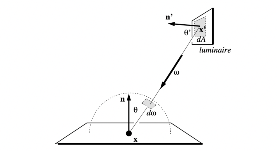
where $\theta'$ is the angle between the light surface normal and the connecting direction.
Substituting into the rendering equation:
$$ L_o(x, \omega_o) = \int_A L_i(x, \omega_i) \, f_r(x, \omega_i, \omega_o) \, \frac{\cos\theta \cos\theta'}{\|x' - x\|^2} \, dA $$Now it is an integral over the light’s area.
The final path tracing algorithm (splitting direct and indirect lighting):
shade(p, wo):
    # direct lighting: sample the light (no RR needed)
    L_direct = 0.0
    uniformly sample a point x' on the light, pdf_light = 1/A
    shoot ray r(p, x')
    if ray is not blocked:
        L_direct = L_i * f_r * cos_theta * cos_theta' / |x'-x|^2 / pdf_light

    # indirect lighting: sample the hemisphere (RR needed)
    L_indirect = 0.0
    uniformly pick ksi in [0,1]
    if (ksi <= P_RR):
        randomly pick 1 direction wi ~ pdf
        shoot ray r(p, wi)
        if ray hits object q:
            L_indirect = shade(q, -wi) * f_r * cos / pdf / P_RR

    return L_direct + L_indirect
Path Tracing in Summary
Path tracing is the core algorithm of modern rendering:
| Property | Description |
|---|---|
| Correctness | Based on the rendering equation — physically correct |
| Global illumination | Naturally supports multiple light bounces |
| Unbiased | Monte Carlo integration guarantees unbiasedness |
| Efficiency | Optimised with RR and direct light sampling |
| Quality | The higher the SPP (samples per pixel), the more accurate the result |
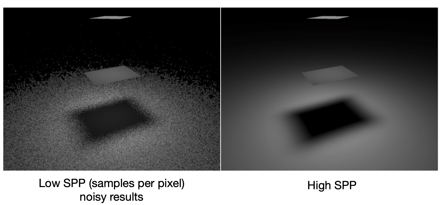
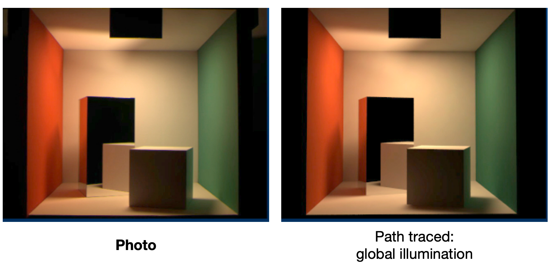
Is path tracing correct? Yes — almost 100% correct, i.e. photo-realistic. A real photograph of the Cornell box and its path-traced global illumination render are nearly indistinguishable.
Ray Tracing: The Old and the New Concept
| Concept | Definition |
|---|---|
| Old | Ray tracing = Whitted-style ray tracing |
| New | The general solution to light transport, including (uni-/bi-directional) path tracing, photon mapping, MLT, VCM/UPBP and more |
Topics Not Covered in the Course
- How do you sample the hemisphere uniformly? How do you generalise to sampling arbitrary functions? (sampling)
- Monte Carlo accepts any PDF — which one is optimal? (importance sampling)
- Does the quality of random numbers matter? (low discrepancy sequences)
- Can sampling the hemisphere and the light be combined? (multiple importance sampling)
- Why is a pixel’s radiance the average radiance of all paths through it? (pixel reconstruction filter)
- Is a pixel’s radiance the pixel’s colour? — No (gamma correction, curves, colour spaces)
Summary
This post covered the core of the GAMES101 ray tracing block:
| Topic | Key points |
|---|---|
| Why ray tracing | Rasterization handles only direct lighting; it cannot do soft shadows, reflection, refraction or GI |
| Ray casting | Appel 1968, pinhole camera model, local lighting only |
| Whitted-style | Recursive reflected/refracted rays, but not physically correct |
| Intersection tests | Sphere (quadratic), plane, implicit surfaces, triangle (Möller–Trumbore) |
| Bounding boxes & slab method | AABB tests, $t_{enter} < t_{exit}$ and $t_{exit} \geq 0$ |
| Acceleration structures | Uniform grids, KD-Tree (spatial) and BVH (object — most common) |
| Radiometry | Energy, flux, intensity, irradiance, radiance; solid angle, Lambert’s cosine law |
| BRDF & reflection equation | A material is a BRDF; outgoing radiance integrates over all incident directions |
| Rendering equation | $L = E + KL$; the series solution shows rasterization stops at $E + KE$ |
| Probability & Monte Carlo | Expectation, PDF, unbiased estimation — estimating integrals by sampling |
| Path tracing | $N = 1$ avoids ray explosion, RR terminates recursion, direct light sampling reduces noise |
This post is note #7 in the GAMES101 - Modern Computer Graphics learning series.