Instructor: Lingqi Yan | UCSB Bilibili: https://www.bilibili.com/video/BV1X7411F744
Rasterization is the process of converting vector graphics (geometric descriptions) into pixel images (raster images).
Rasterization = drawing continuous geometry as discrete pixels. It is the foundational technique of real-time rendering.
This chapter corresponds to lectures 5-6 (the depth buffer part corresponds to the start of lecture 7).
1 Perspective Projection Wrap-Up: fovY and Aspect Ratio
In the MVP transform, the perspective projection frustum is defined by $l, r, b, t$ (left, right, bottom, top bounds of the near clip plane), but in practice developers prefer vertical field of view (fovY) and aspect ratio (assuming symmetry, i.e. $l = -r$, $b = -t$):
| Parameter | Meaning |
|---|---|
| fovY | Vertical field of view: the angle the visible range opens in the vertical direction from the camera |
| aspect ratio | Width / height: $\text{aspect} = \dfrac{\text{width}}{\text{height}}$ |
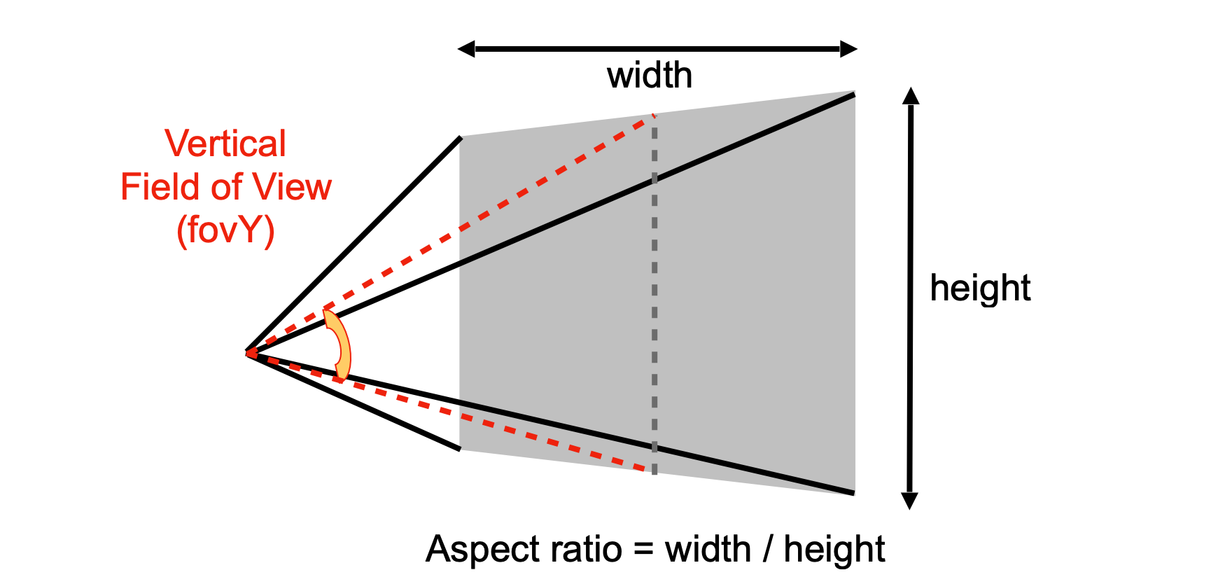
Converting between fovY / aspect and $l, r, b, t$ (derived directly from the triangle relations on the near clip plane):
$$ \tan\frac{fovY}{2} = \frac{t}{|n|} \qquad\qquad \text{aspect} = \frac{r}{t} $$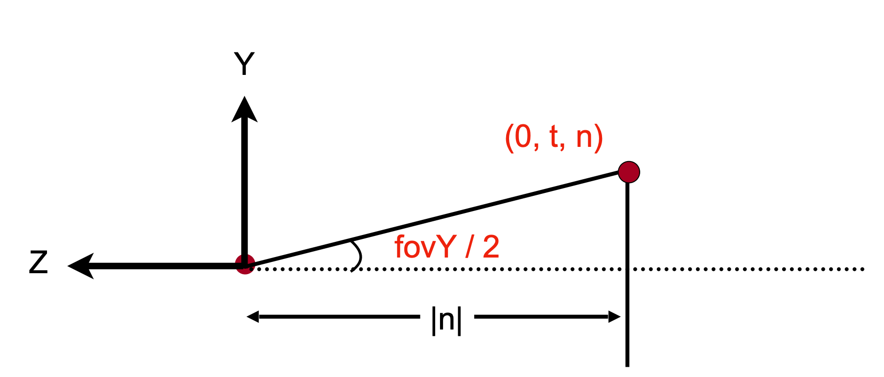
Given fovY and the near plane distance $n$, we can compute $t$, then derive $r$ from the aspect ratio, and by symmetry get $b$ and $l$.
2 Viewport Transformation
What Comes After MVP
- Model transformation (place objects)
- View transformation (place the camera)
- Projection transformation
- Orthographic projection: cuboid → canonical cube $[-1,1]^3$
- Perspective projection: frustum → canonical cube
- One last step remains: canonical cube → screen
What Is a Screen
- A screen is an array of pixels
- Array size = resolution
- Raster (German) = screen, Rasterize = rasterization = drawing onto the screen
- Pixel: short for “picture element”. Each pixel is a small square whose color is an RGB blend
Screen Space Definition
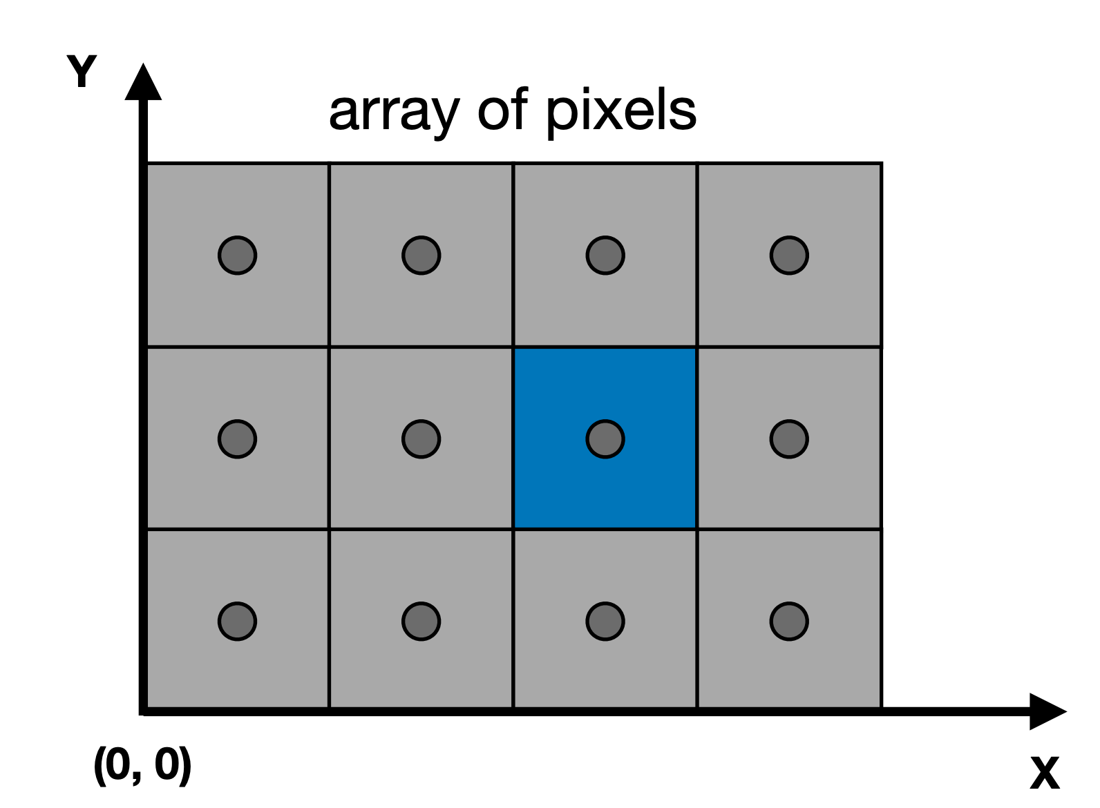
| Property | Description |
|---|---|
| Pixel index range | $(0, 0)$ to $(width-1, height-1)$ |
| Pixel center | The center of pixel $(x, y)$ is at $(x+0.5, y+0.5)$ |
| Screen coverage | $(0, 0)$ to $(width, height)$ |
Viewport Transformation Matrix
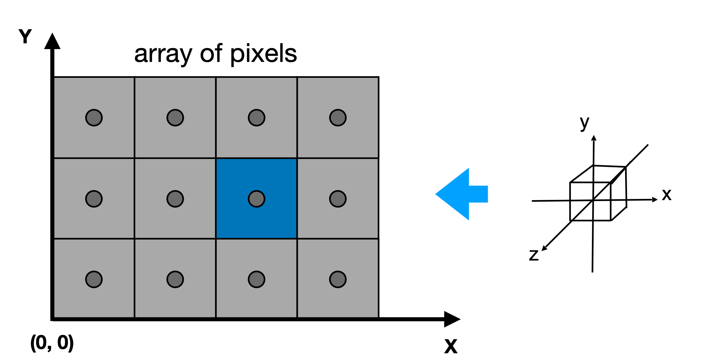
Transform the canonical cube $[-1,1]^2$ to screen space $[0, width] \times [0, height]$:
$$ M_{viewport} = \begin{pmatrix} \frac{width}{2} & 0 & 0 & \frac{width}{2} \\ 0 & \frac{height}{2} & 0 & \frac{height}{2} \\ 0 & 0 & 1 & 0 \\ 0 & 0 & 0 & 1 \end{pmatrix} $$Note: This transformation is independent of z; it works only in the xy plane, combining translation and scaling.
3 Raster Displays
Before “drawing to the screen”, let’s look at what kinds of “screens” exist.
Drawing Machines
- CNC Sharpie Drawing Machines, laser cutters, etc. are devices that “draw” graphics with discrete control.


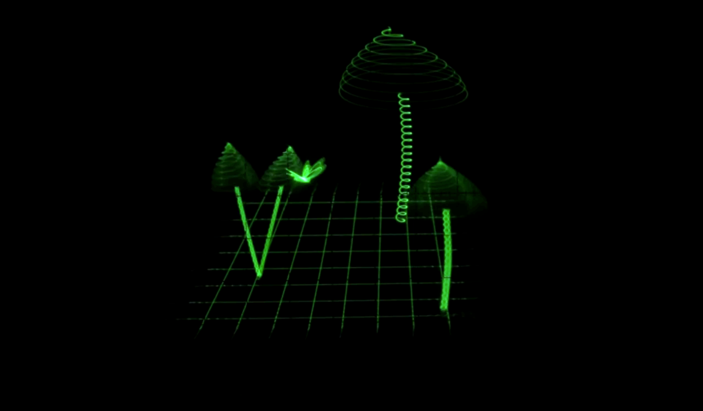
Oscilloscope
- Deflects an electron beam to “draw lines” directly; can also create Oscilloscope Art.

Cathode Ray Tube (CRT)
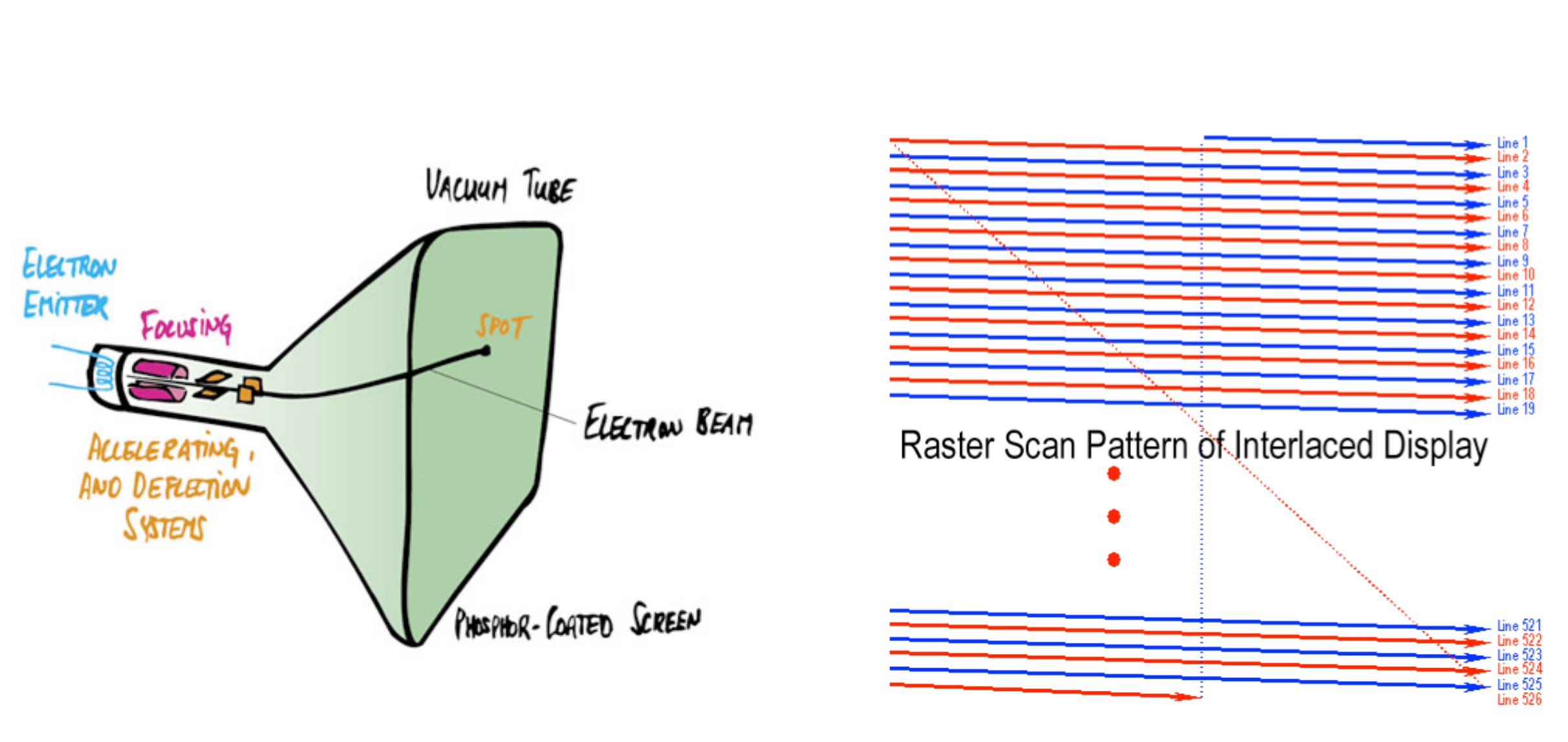
- Raster Scan: the electron beam scans line by line from left to right and top to bottom, modulating intensity to control brightness.
- Interlaced scanning (odd lines then even lines) was a bandwidth optimization of the CRT era.
Frame Buffer
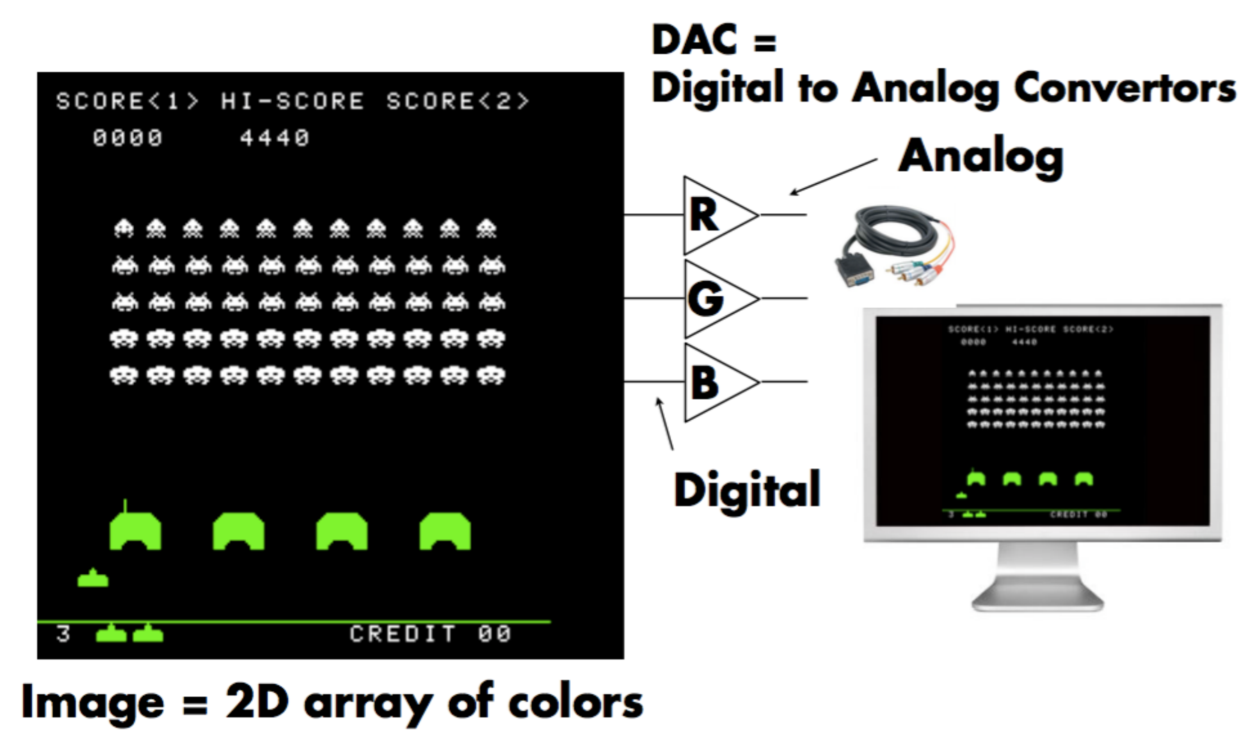
- A chunk of memory provided for raster displays.
- The GPU/display device reads pixel values directly from the frame buffer and shows them on the screen.
Flat Panel Displays
| Type | Principle |
|---|---|
| LCD (Liquid Crystal Display) | Twisting liquid crystals changes polarization to block or transmit light; lit by backlight (fluorescent or LED), partial twisting yields intermediate grays |
| LED Array Display | An array of light-emitting diodes, each LED emits directly (large outdoor screens) |
| E-ink (Electrophoretic Display) | Electric fields move charged pigment particles to show colors; the image persists after power-off, but switching takes time (e.g. Kindle) |


4 Why Triangles
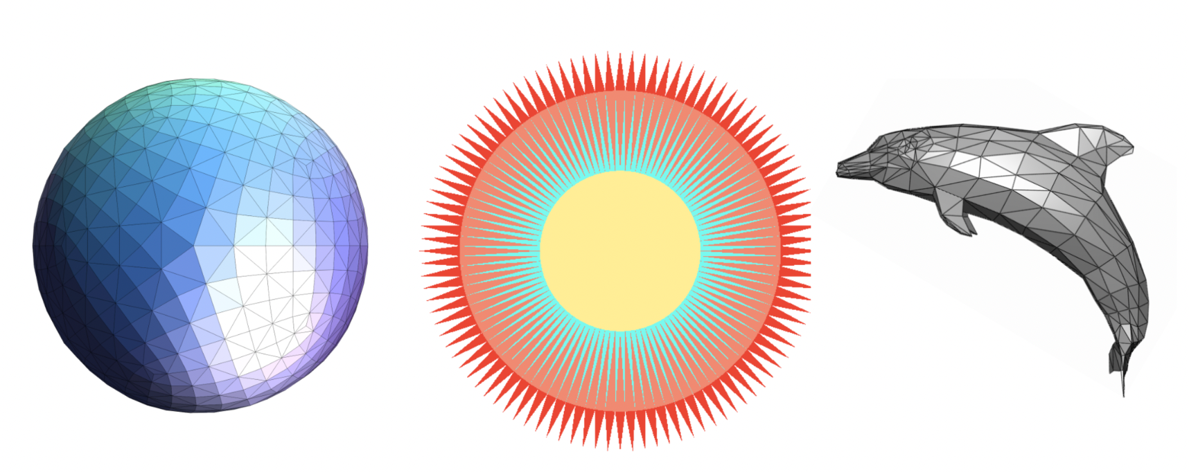
Triangles are the most basic primitive and have unique advantages in graphics:
| Property | Description |
|---|---|
| Most basic polygon | Any polygon can be decomposed into triangles |
| Guaranteed coplanar | Three points define a plane |
| Well-defined inside/outside | There is a clear way to test whether a point is inside a triangle |
| Well-defined interpolation | Can interpolate across vertices (barycentric coordinates) |
Input and output of rasterizing a triangle:
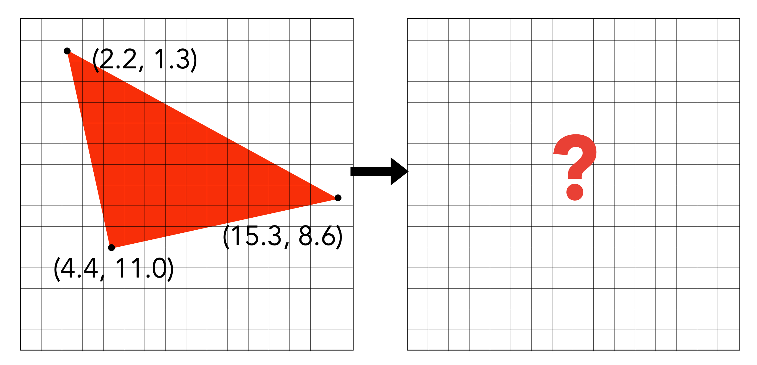
- Input: the screen-space positions of the three projected triangle vertices (floating-point coordinates)
- Output: a set of pixel values that approximate the triangle coverage
Core idea: determine the positional relationship between each pixel and the triangle, considering the pixel center relative to the triangle.
5 Sampling and Point-in-Triangle Test
Basic Idea
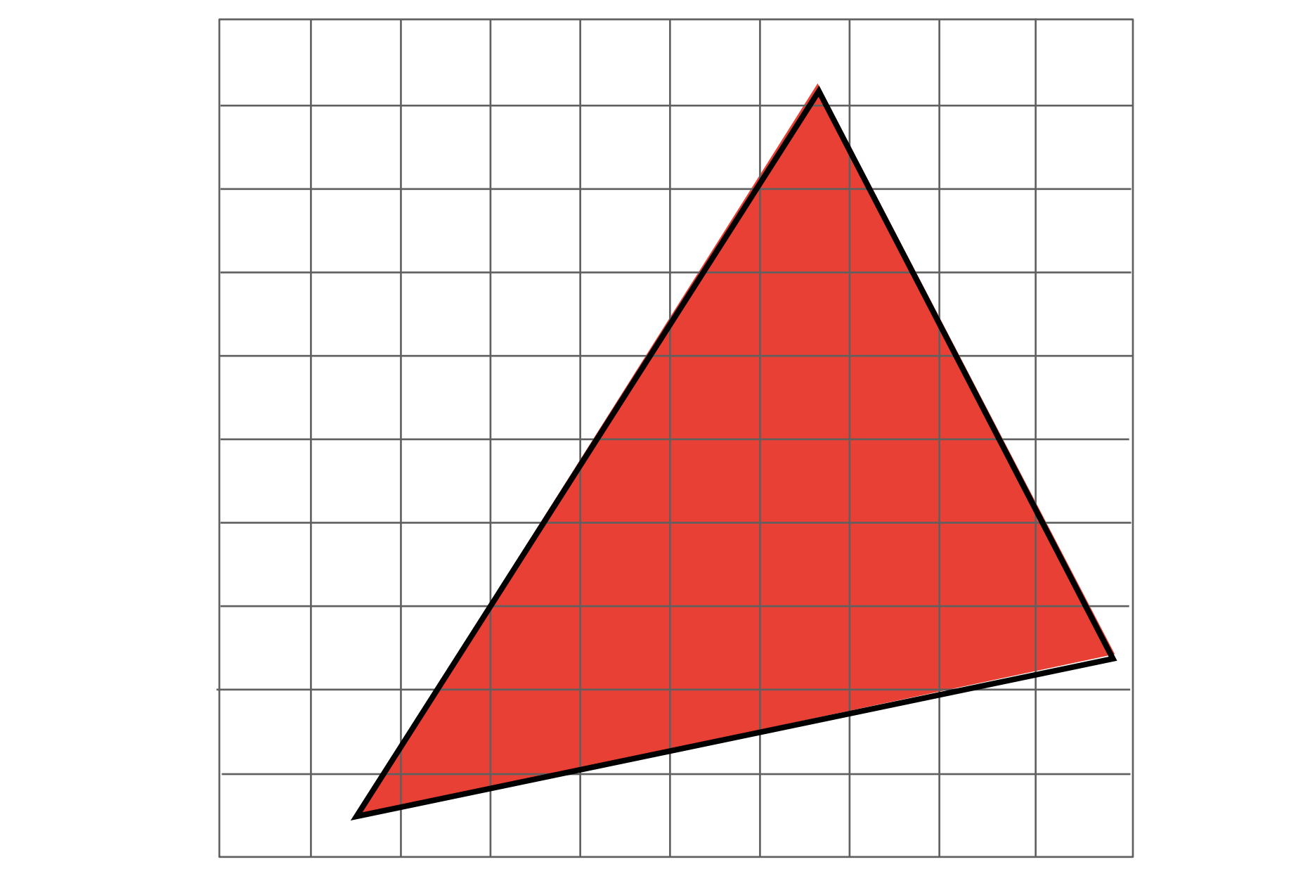
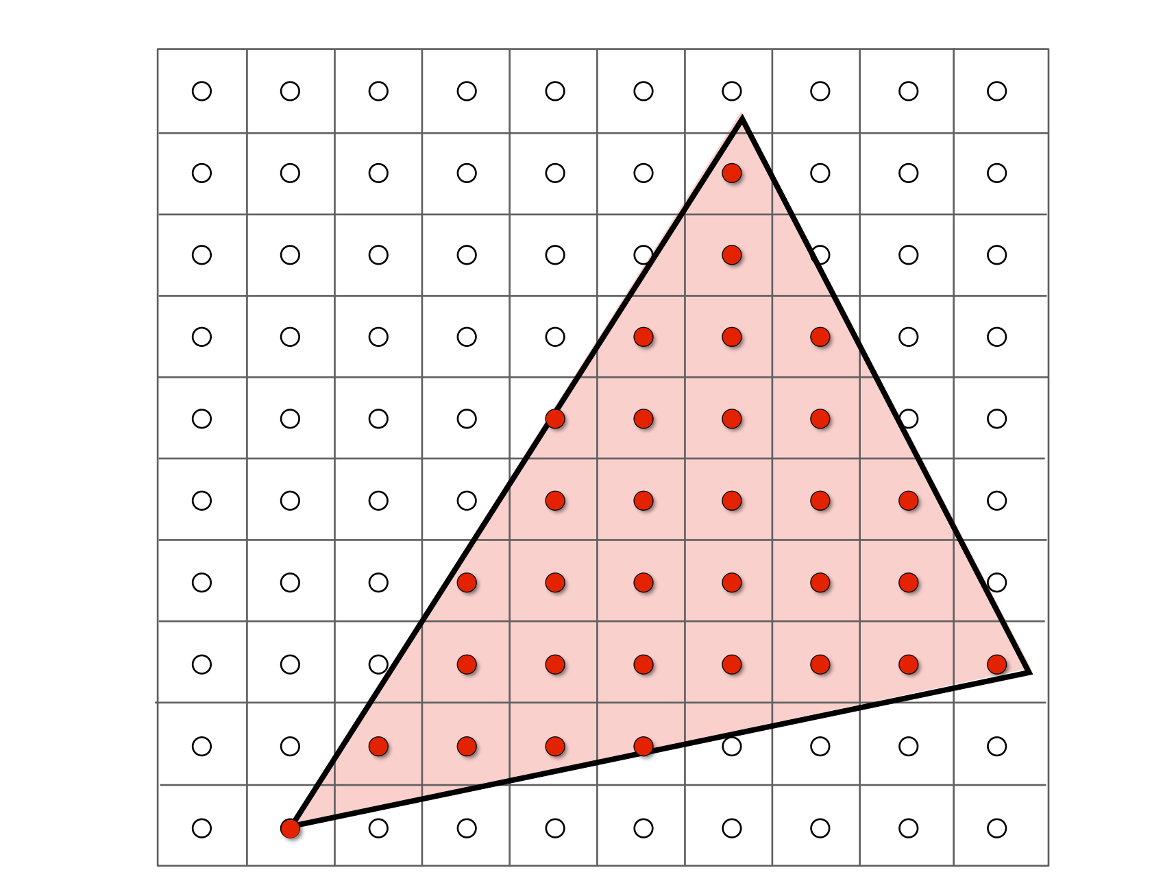
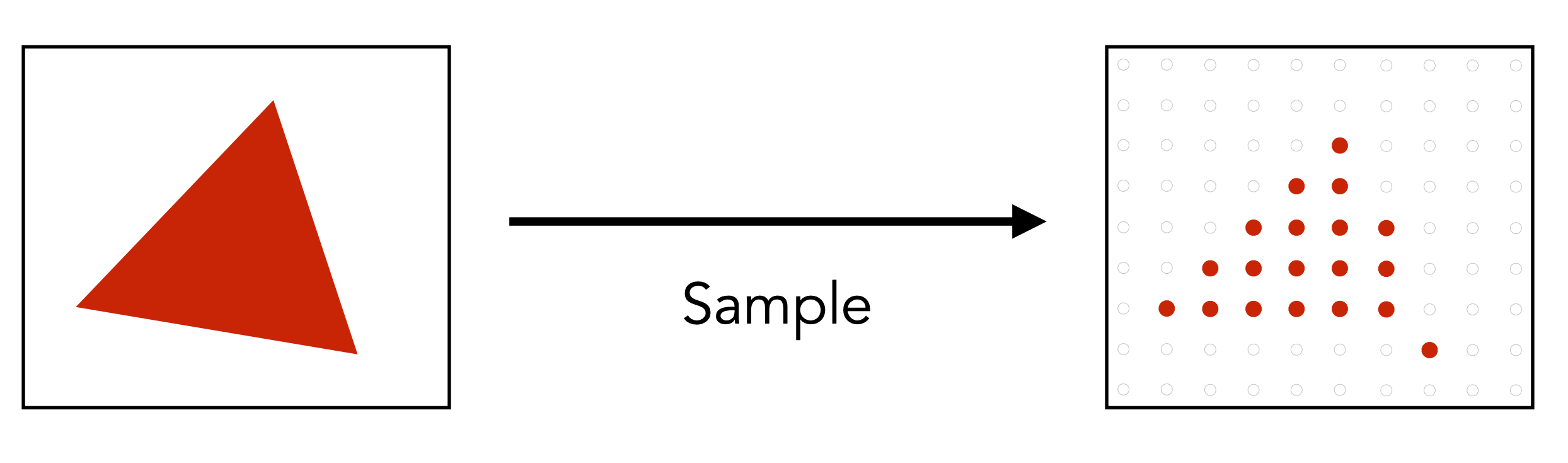
Rasterization is essentially sampling a triangle:
- For each pixel center on the screen, test whether it is inside the triangle.
- Define a binary function:
Sampling Code
for (int x = 0; x < xmax; ++x)
    for (int y = 0; y < ymax; ++y)
        image[x][y] = inside(tri, x + 0.5, y + 0.5);
Note: The sampling position is the pixel center $(x+0.5, y+0.5)$, not $(x, y)$.
Cross-Product Point-in-Triangle Test
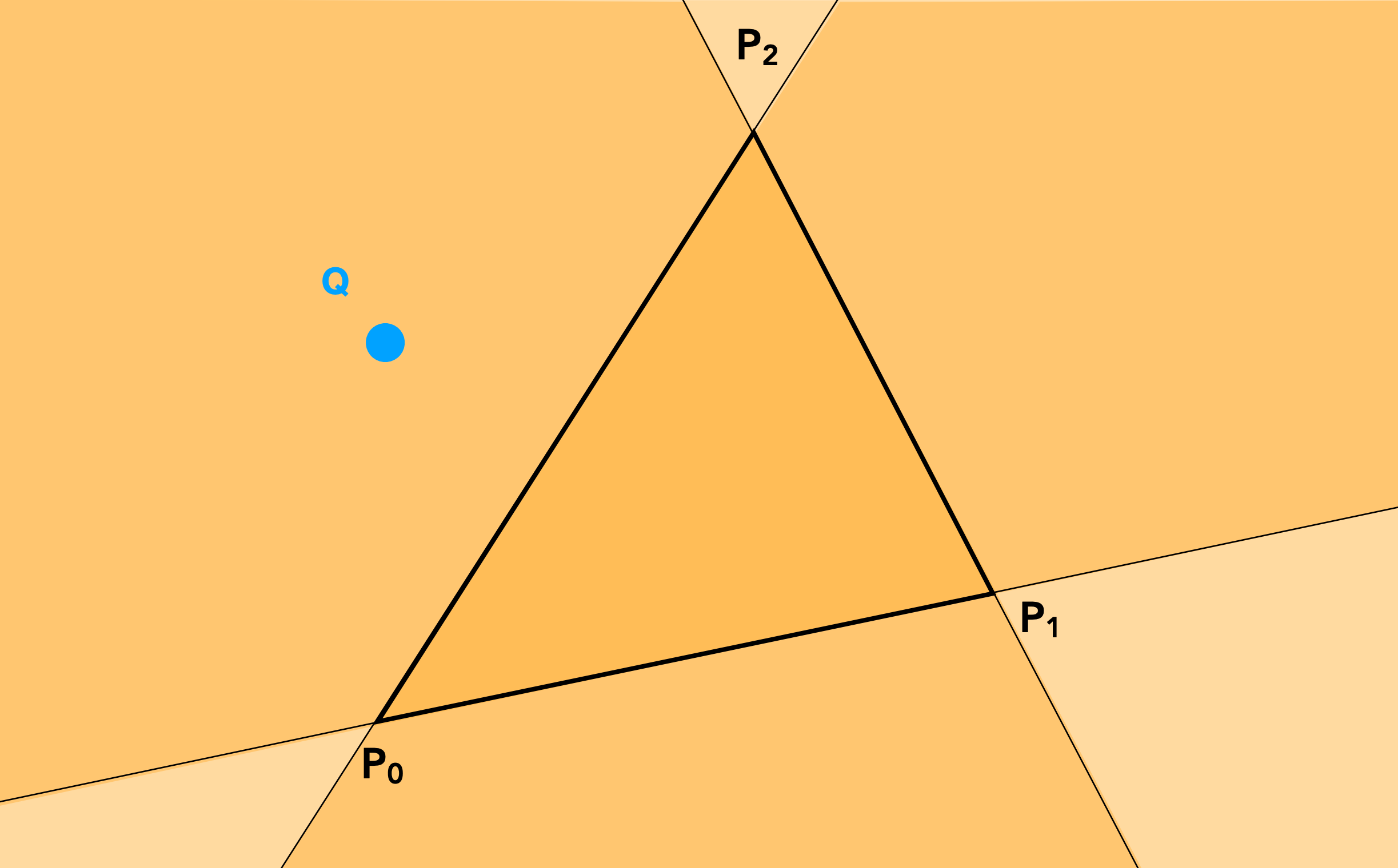
Using the cross product to test whether point P is inside triangle ABC (as in the vector chapter):
bool insideTriangle(float x, float y, const Vector3f* _v) {
    // Compute the cross product for each edge AB, BC, CA
    // If P is on the same side (left side) of all three edges, P is inside the triangle
    Vector3f P(x, y, 0);

    // Compute the three edge vectors
    Vector3f AB = _v[1] - _v[0];
    Vector3f BC = _v[2] - _v[1];
    Vector3f CA = _v[0] - _v[2];

    // Compute vectors from vertices to P
    Vector3f AP = P - _v[0];
    Vector3f BP = P - _v[1];
    Vector3f CP = P - _v[2];

    // Cross products to determine direction
    float z1 = cross(AB, AP).z;
    float z2 = cross(BC, BP).z;
    float z3 = cross(CA, CP).z;

    // Same sign means inside the triangle
    return (z1 > 0 && z2 > 0 && z3 > 0) || (z1 < 0 && z2 < 0 && z3 < 0);
}
Edge Cases
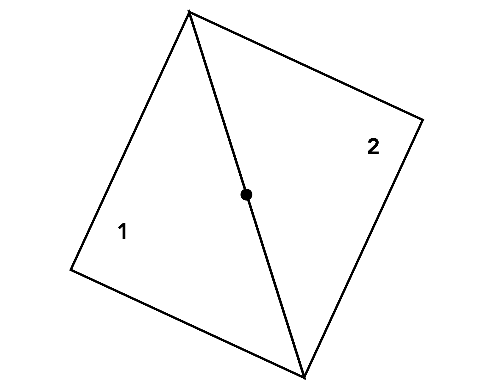
When a sample point lies exactly on a triangle edge (two triangles share an edge), special handling is needed:
- Convention: points on the edge count as inside.
- Or: only on specific edges count (e.g. left and top boundaries).
- The course adopts a lenient policy: no special handling — not covering it is not wrong either.
6 Bounding Box Optimization
Problem
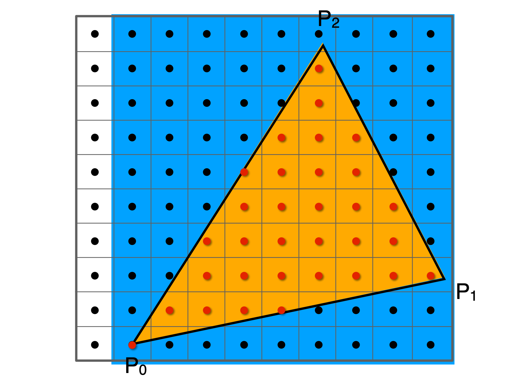
Scanning every pixel on the screen is inefficient; most pixels are outside the triangle.
Solution
Use the triangle’s axis-aligned bounding box (AABB) to limit the sampling range:
// Compute the bounding box
int minX = max(0, min(v0.x, min(v1.x, v2.x)));
int maxX = min(width - 1, max(v0.x, max(v1.x, v2.x)));
int minY = max(0, min(v1.y, min(v0.y, v2.y)));
int maxY = min(height - 1, max(v0.y, max(v1.y, v2.y)));

// Sample only inside the bounding box
for (int x = minX; x <= maxX; ++x)
    for (int y = minY; y <= maxY; ++y)
        if (insideTriangle(x + 0.5, y + 0.5, vertices))
            image[x][y] = color;
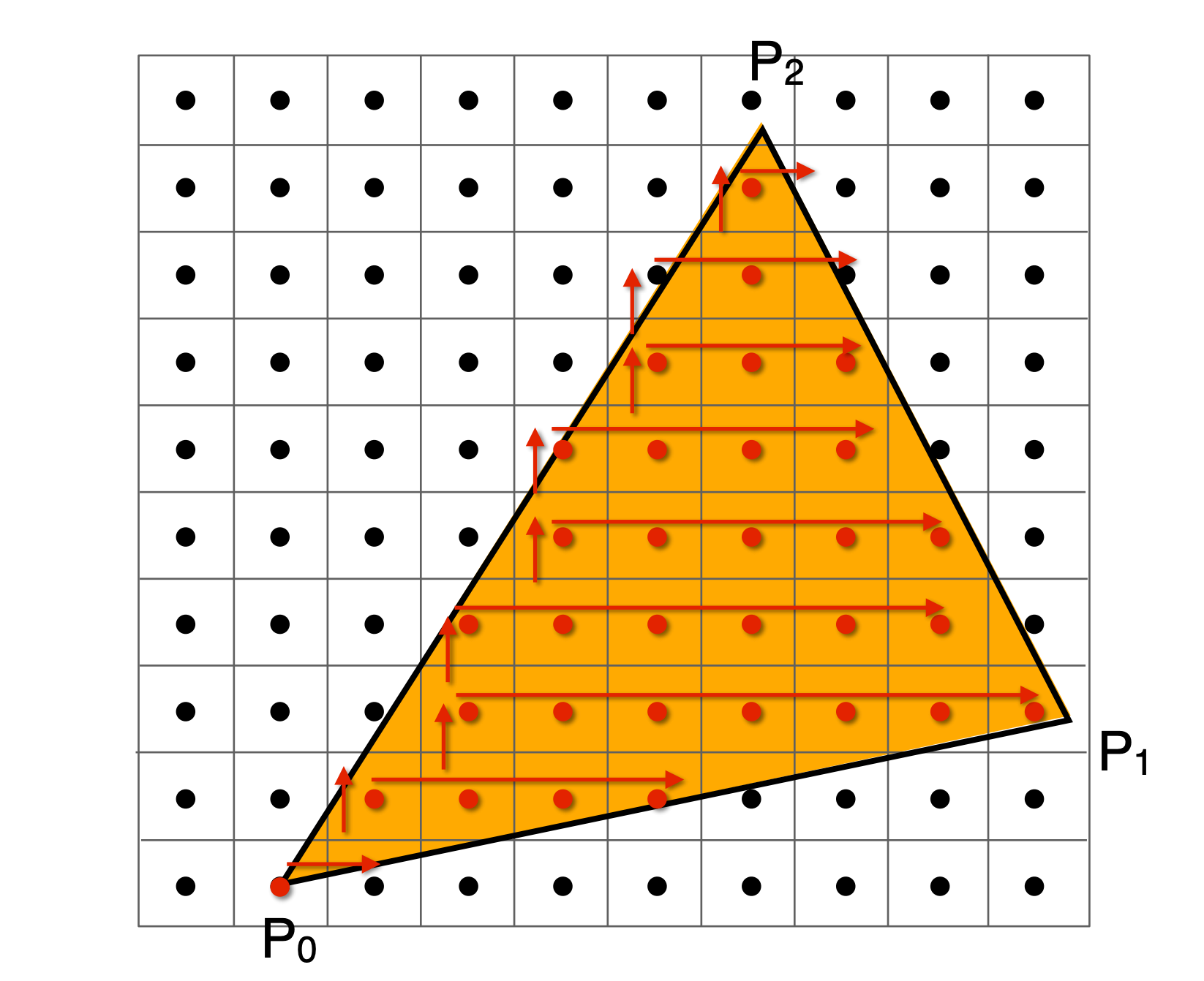
For thin or rotated triangles, Incremental Triangle Traversal can further optimize: start from the leftmost pixel of the triangle, advance row by row reusing the previous row’s result, and traverse only the pixels actually covered.
7 Rasterization on Real Display Devices
What Real Pixels Look Like
Zooming into real LCD screens (iPhone 6S, Galaxy S5), each pixel consists of R, G, B subpixels, and different vendors arrange subpixels (pixel geometry) differently.

Notice there are more green subpixels than red and blue — because the human eye is most sensitive to green. More green sensors make the image look more comfortable and natural.
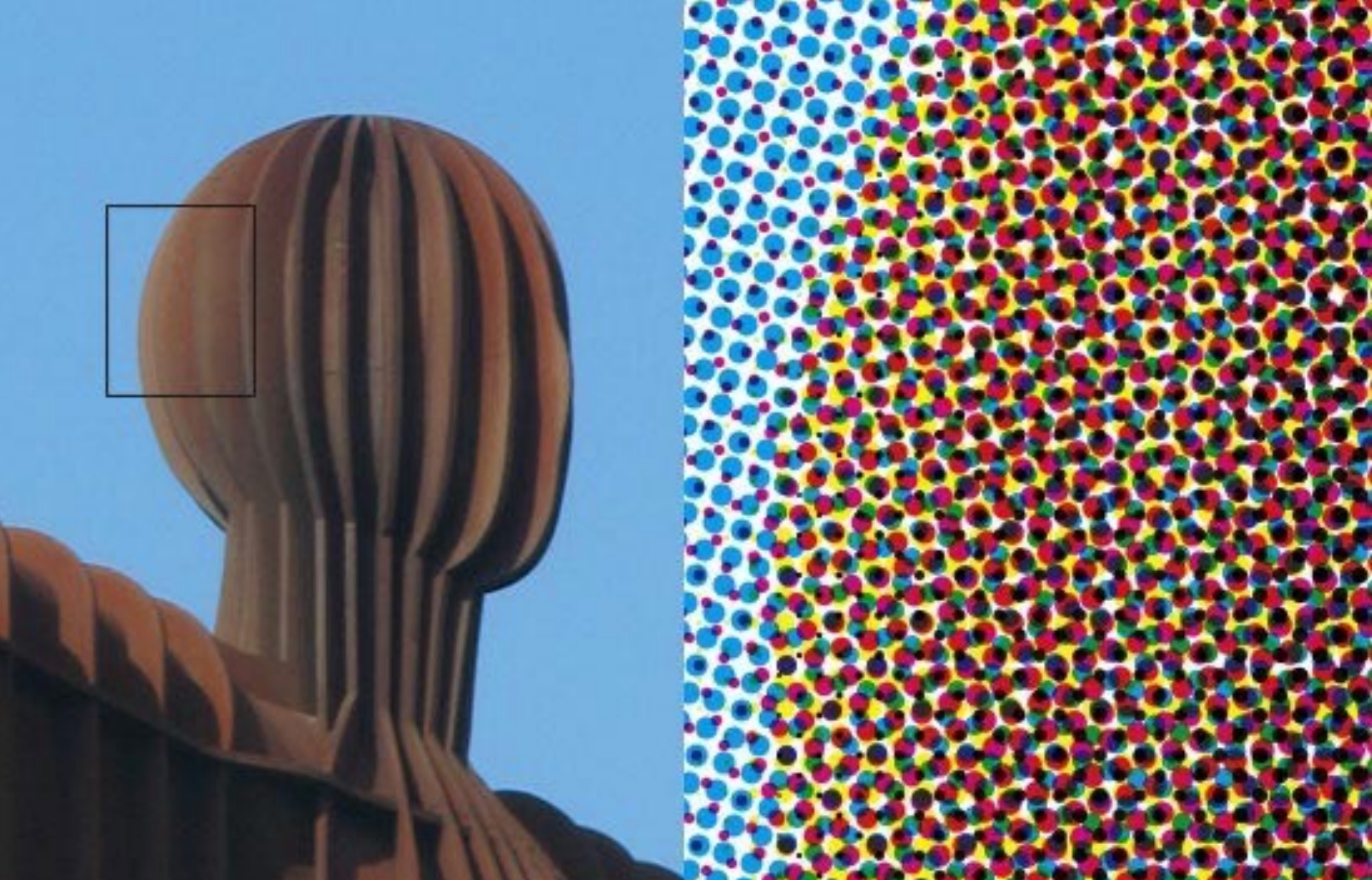
Color printing approximates continuous color using half-tone patterns (dots of varying density).
Assumptions in This Course
- Assume each pixel emits a square of uniformly colored light (not true for LCD, but a good enough approximation for this course).
- Then send sampling signals (one color per pixel), and the display device physically emits the corresponding signal.
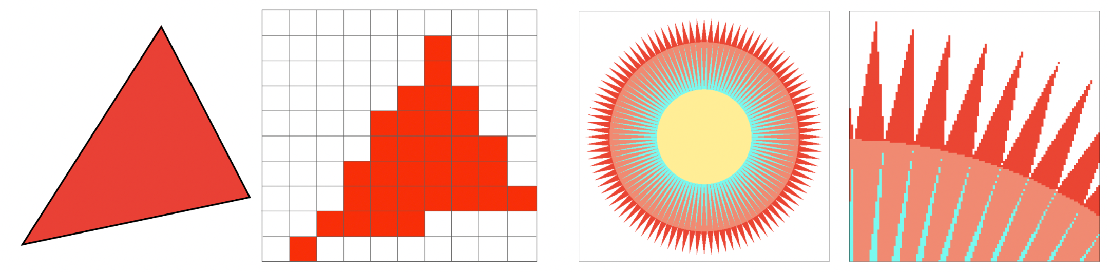
Comparing the sampled signal with the continuous triangle function reveals a serious problem — jaggies.
8 The Aliasing Problem
Sampling Is Everywhere
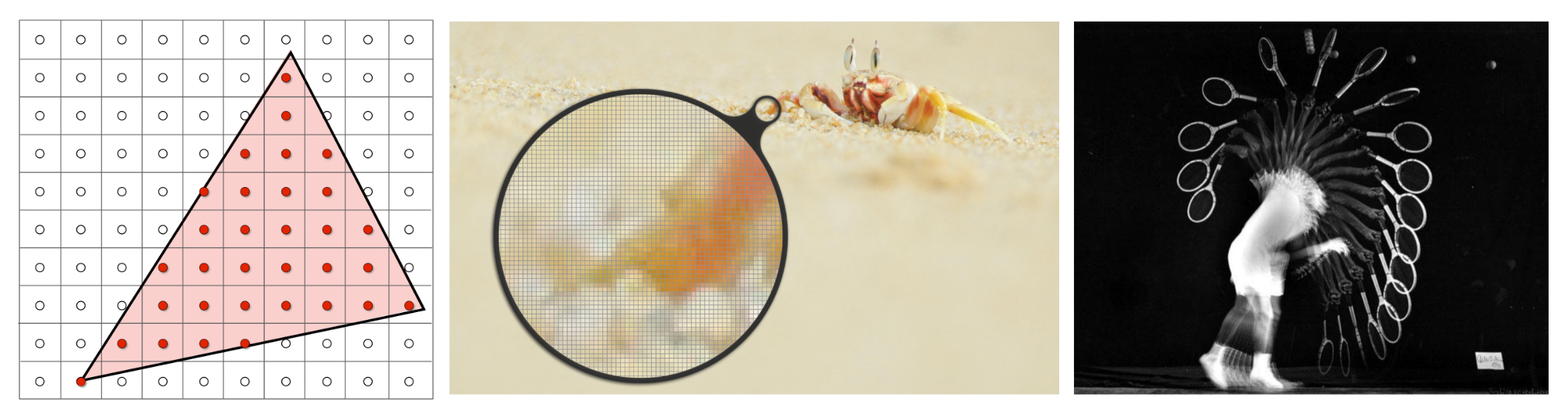
Sampling is a core concept in graphics, appearing everywhere:
| Scenario | What is sampled |
|---|---|
| Rasterization | 2D positions (screen space) |
| Photography | The image sensor plane |
| Video | Time |
What Are Jaggies
Rasterized triangle edges show staircase artifacts (jaggies), caused by undersampling — this is aliasing, one kind of sampling error (Errors / Mistakes / Inaccuracies).
Common Manifestations of Aliasing

| Type | Description | Cause |
|---|---|---|
| Jaggies | Staircase edges in space | Spatial undersampling |
| Moiré | Stripe patterns in images (e.g. shrinking by skipping odd rows/columns) | Image undersampling |
| Wagon Wheel | Apparent reversed motion (wheel spinning backwards illusion) | Temporal undersampling |
Root Cause
The signal changes too fast (high frequency) while sampling is too slow (low frequency).
9 Anti-Aliasing
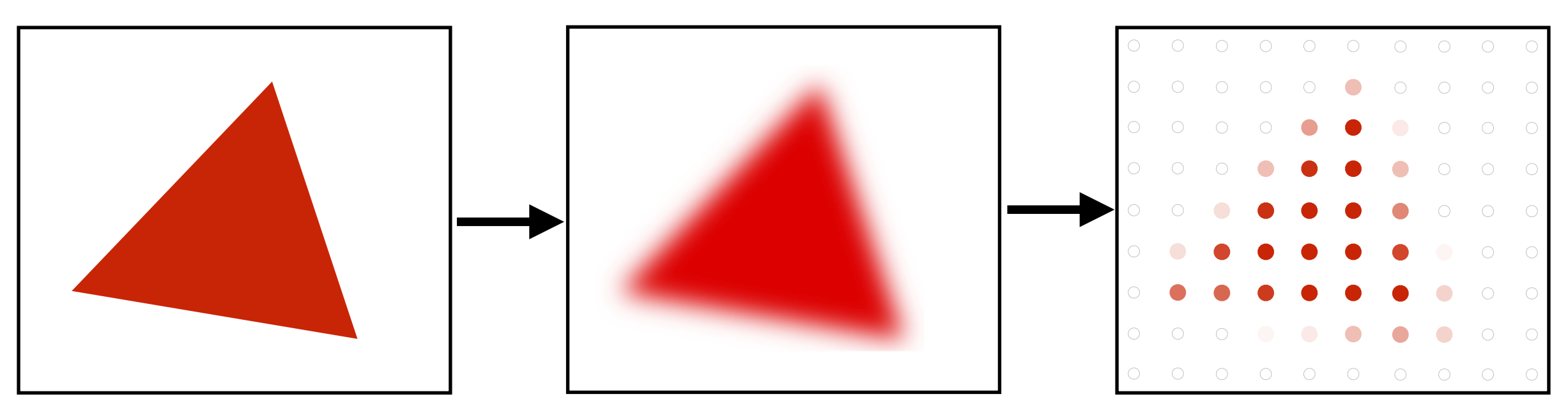
Core Idea: Blur First, Then Sample (Pre-Filtering Before Sampling)
Pre-filter (blur) the triangle before sampling so edge pixels take intermediate values (half red, half white → pink), eliminating jaggies.

Order matters:
- Filter first, then sample (correct!) → smooth edges
- Sample first, then filter (wrong!) → blurred jaggies

Frequency Domain View
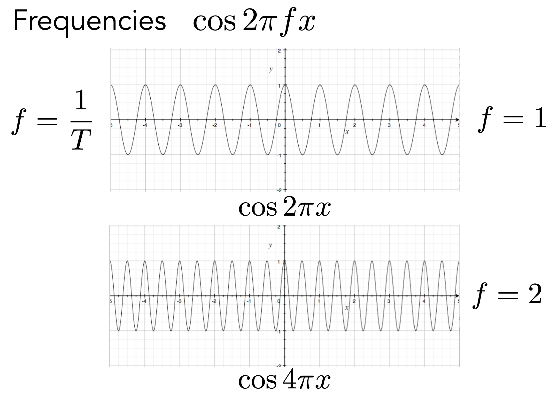
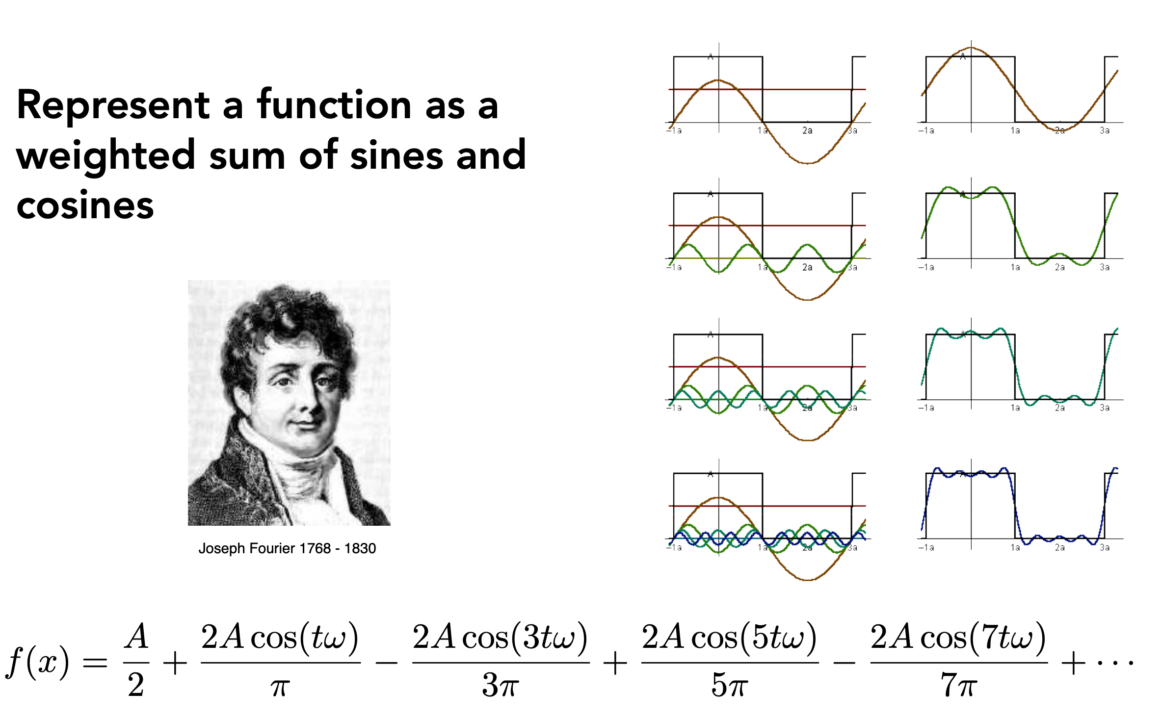
Frequency and sine/cosine: $f = \frac{1}{T}$ (reciprocal of period T). Any signal can be written as a weighted sum of sines/cosines of different frequencies. For example, a square wave can be decomposed as:
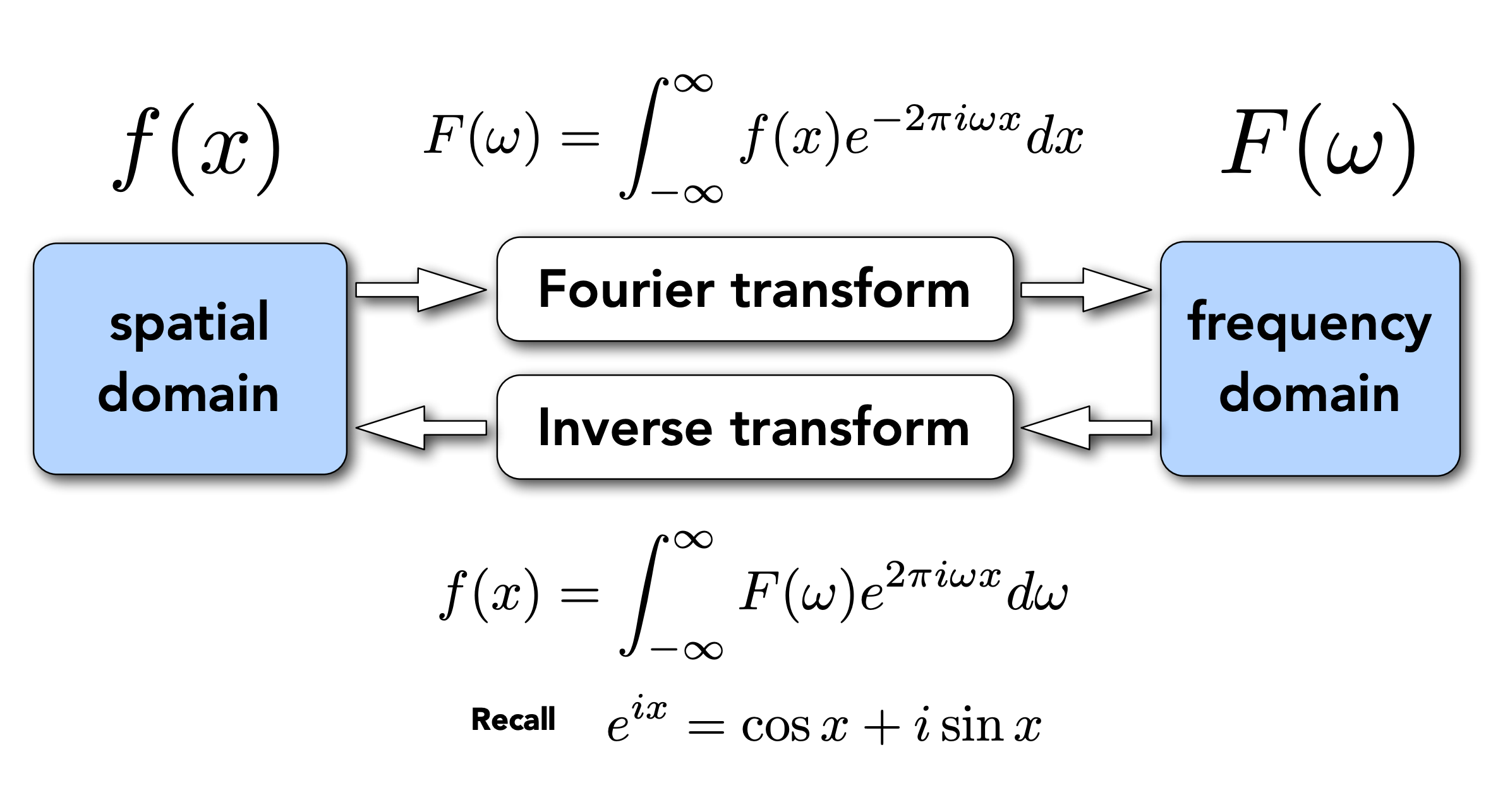
Fourier Transform: decomposes a signal into a weighted sum of sines/cosines of different frequencies (converts between spatial domain and frequency domain).
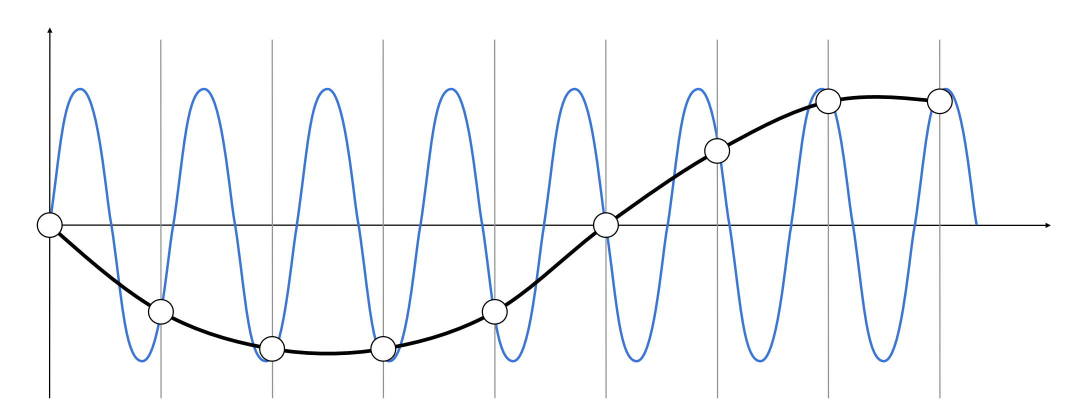
High-frequency signals need faster sampling:
Sampling rate is related to the signal’s frequency.
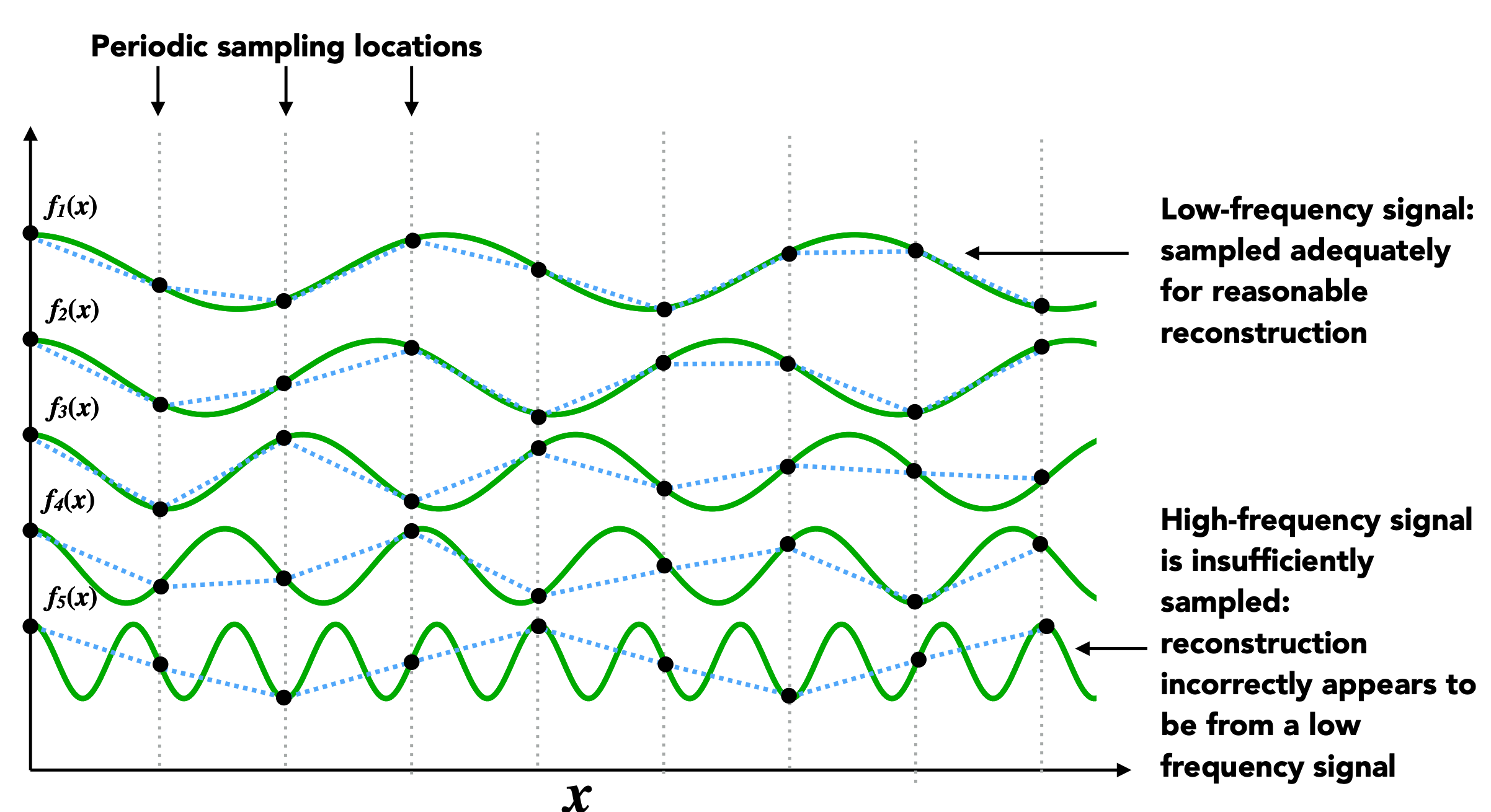
- Low-frequency signals: adequately sampled, can be reconstructed correctly.
- High-frequency signals: undersampled, reconstruction incorrectly masquerades as low frequency.
- Two frequencies indistinguishable at a given sampling rate are called aliases of each other.
Filtering
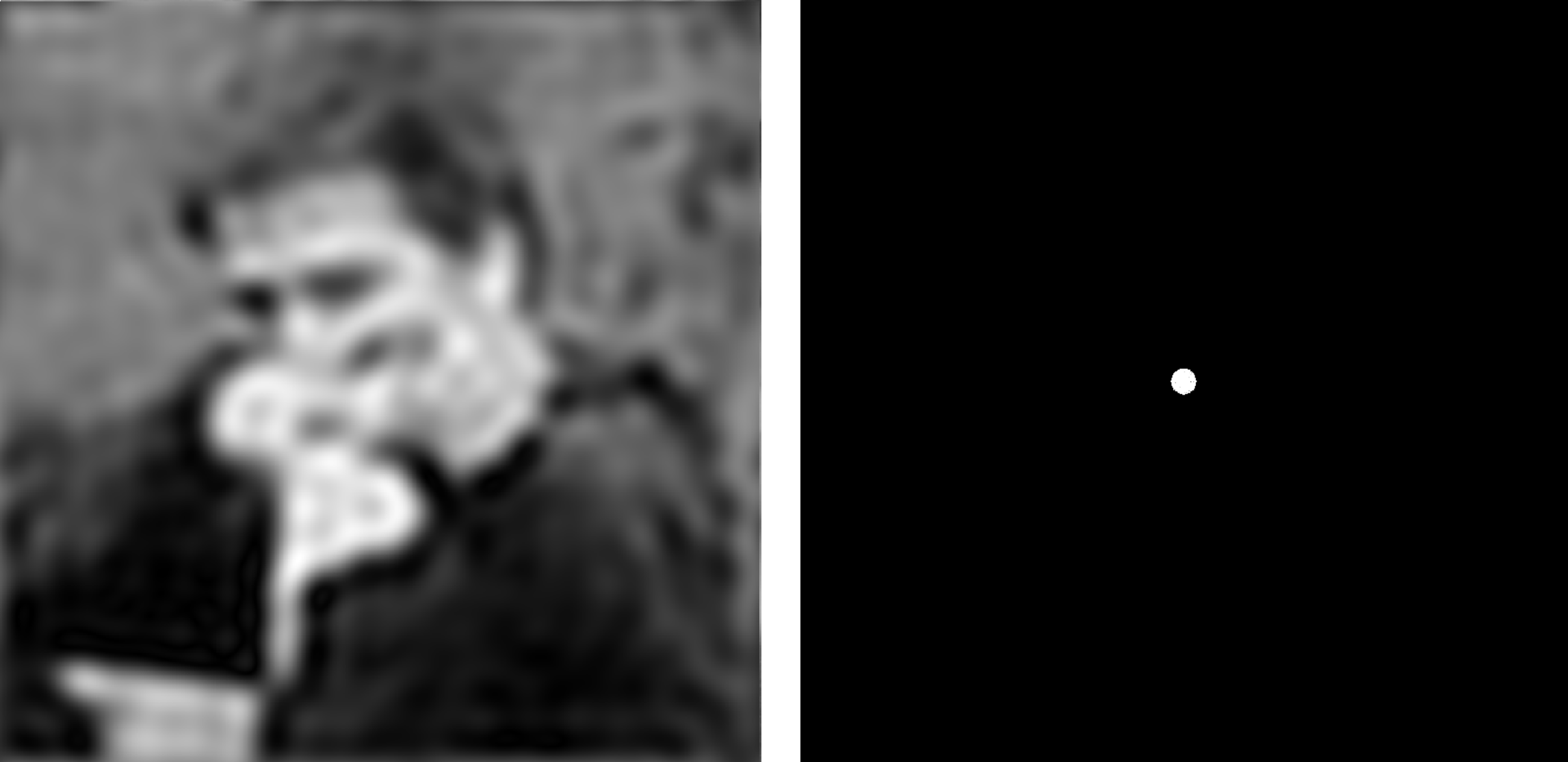
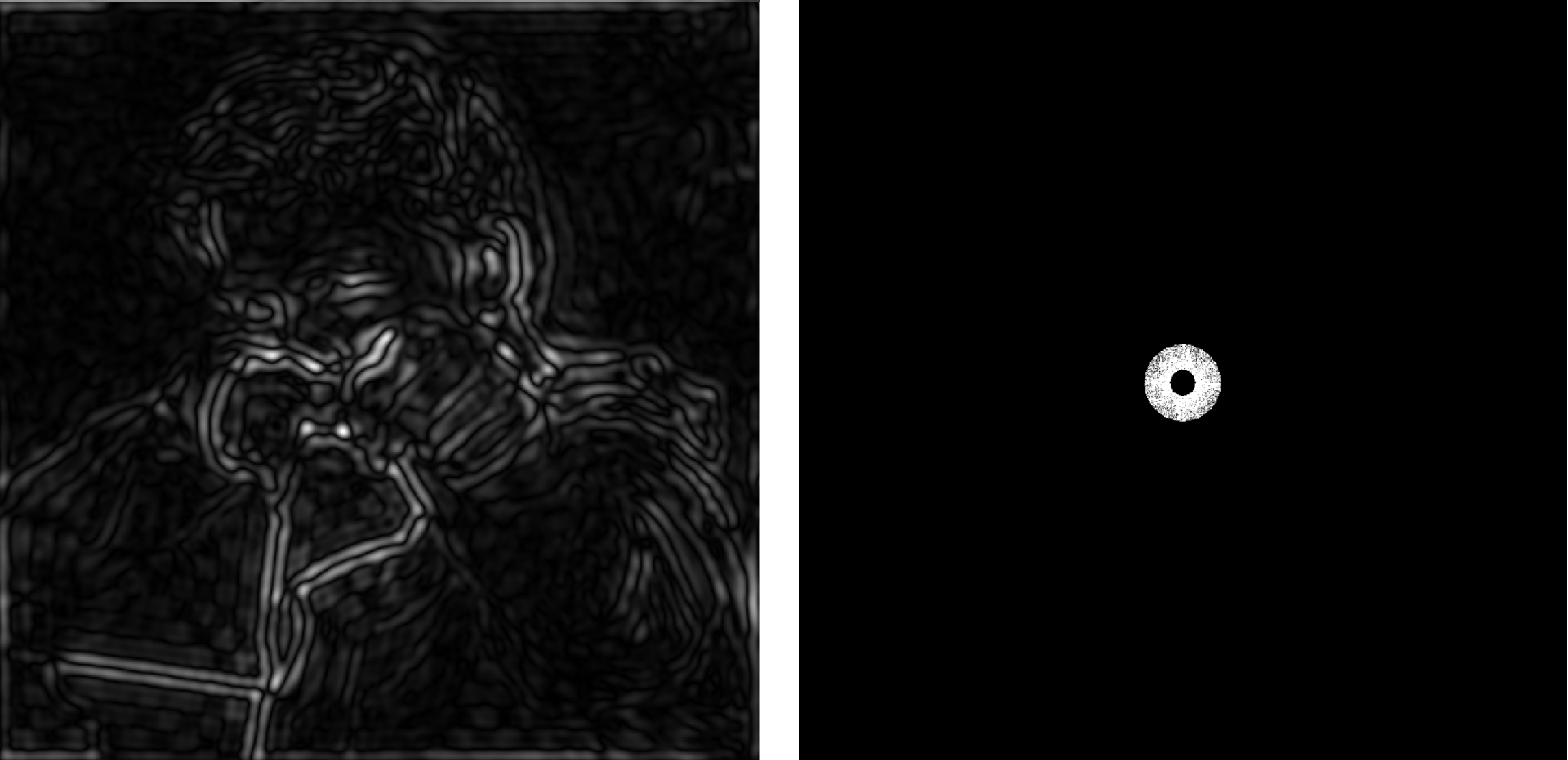
Filtering = removing certain frequency components.

| Filter type | Effect | Frequency domain result |
|---|---|---|
| Low-pass | Blur the image, remove boundaries, remove high frequencies | Keep low frequencies, remove high frequencies |
| High-pass | Extract edges, remove low frequencies | Keep high frequencies, remove low frequencies |
| Band-pass | Keep a specific frequency range | Remove too-high and too-low frequencies |
High-pass filtering: what is an edge? When the image above/below and left/right differ a lot, i.e. drastic changes (high-frequency information).

Convolution: Filtering = Convolution = Averaging
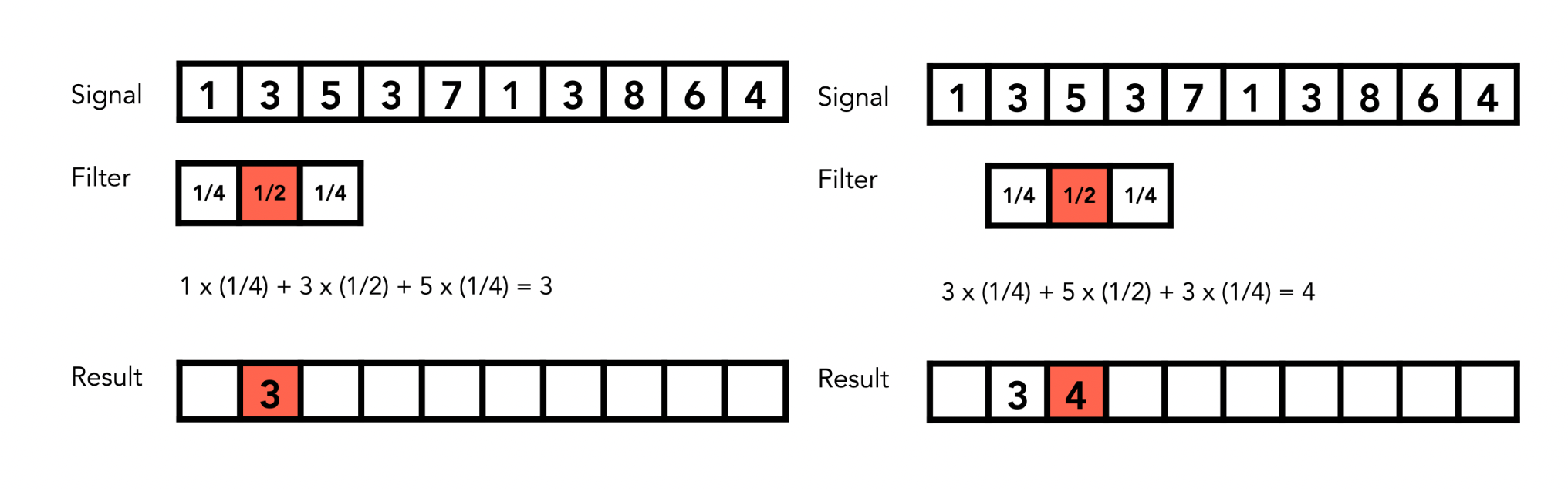
Convolution: pointwise local averaging within a “sliding window” (Convolution = Averaging).
For example, signal [1 3 5 3 7 1 3 8 6 4] with filter [1/4, 1/2, 1/4]:
Step 1:  1×(1/4) + 3×(1/2) + 5×(1/4) = 3
Step 2:  3×(1/4) + 5×(1/2) + 3×(1/4) = 4
...the window slides step by step, producing the output sequence
Convolution theorem: convolution in the spatial domain = multiplication in the frequency domain (and vice versa).
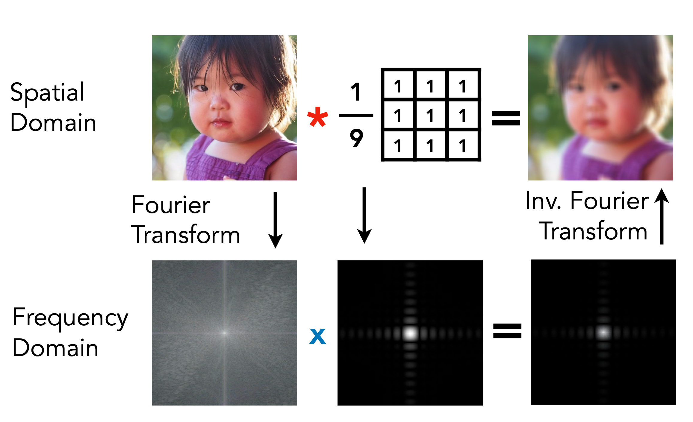
So filtering has two equivalent approaches:
- Convolve directly in the spatial domain.
- Transform to the frequency domain → multiply by the Fourier transform of the kernel → inverse transform back.
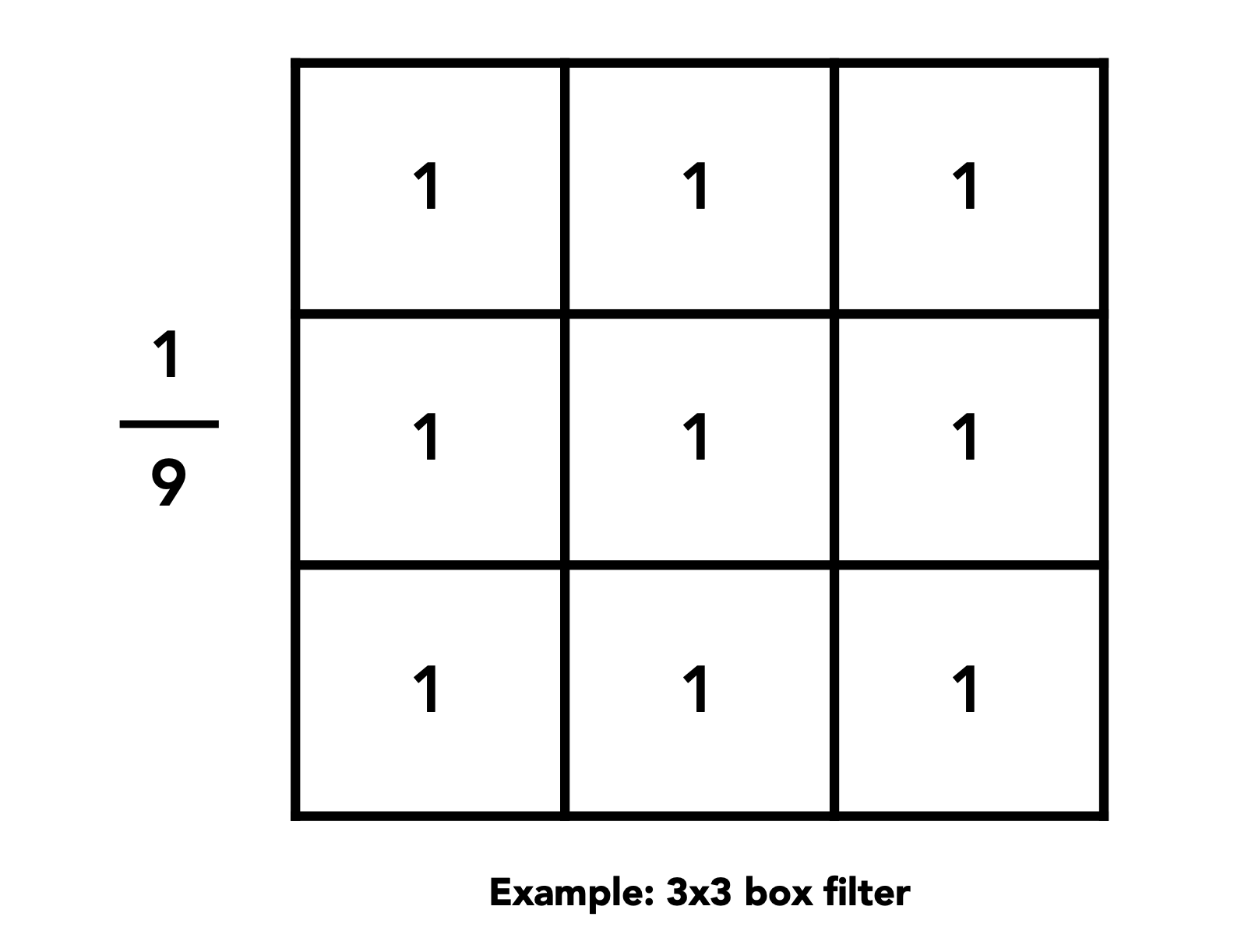
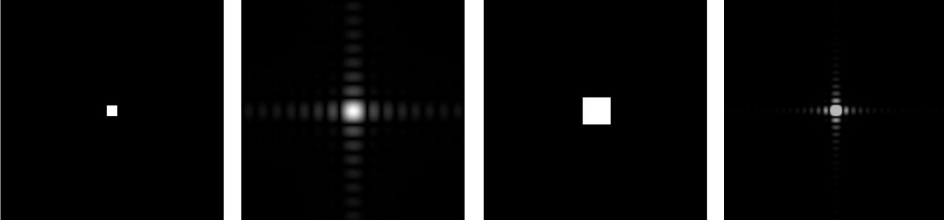
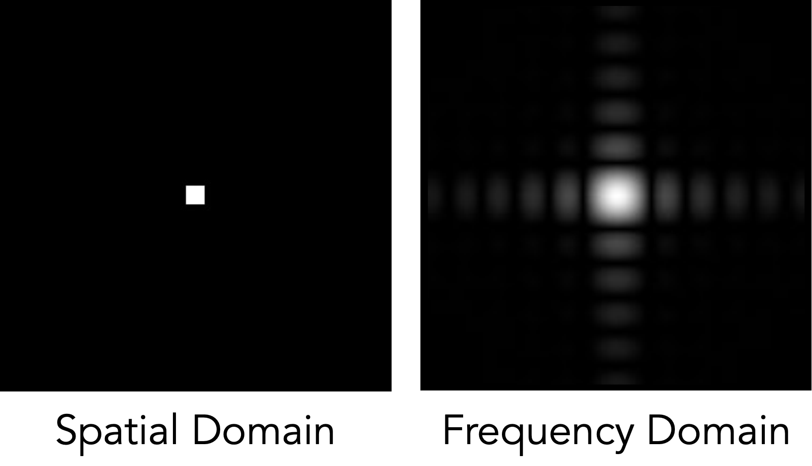
Box Filter: a 1-pixel-wide box filter acts as a low-pass filter (blur).
Wider filter kernel = keep only lower frequencies (blur more).
Sampling = Repeating Frequency Content
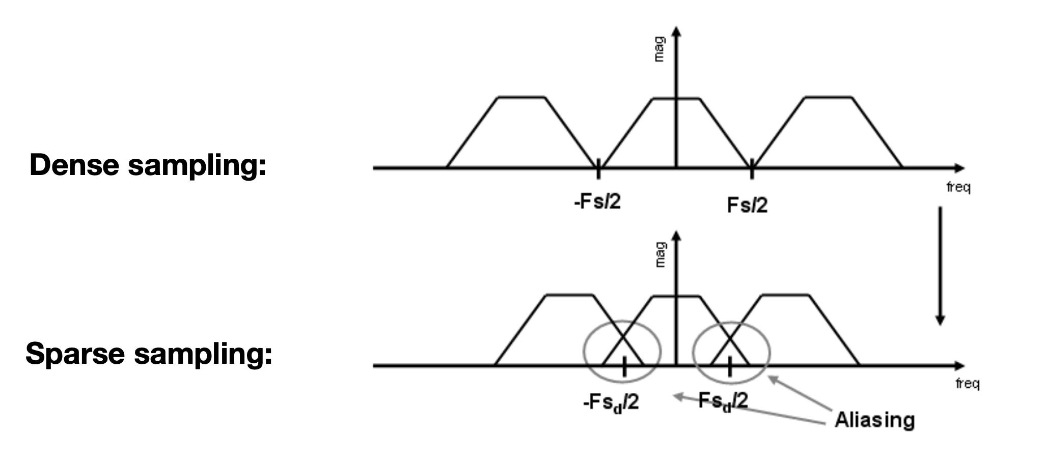
Sampling = repeating frequency content: the higher the sampling rate, the larger the spacing between frequency-domain copies.
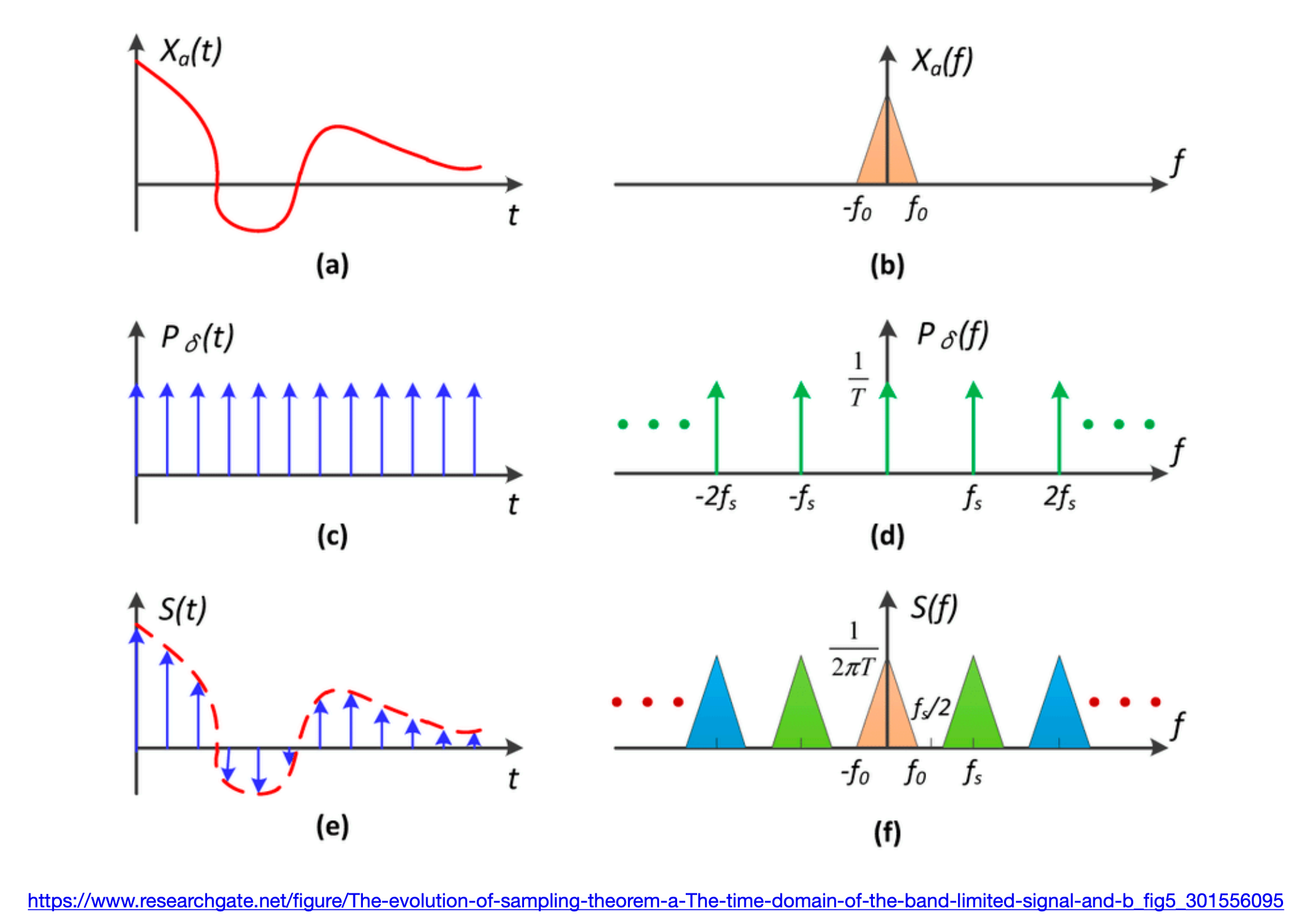
Aliasing = mixing frequency content: undersampling (sparse sampling) causes spectrum copies to overlap, and high frequencies masquerade as low frequencies.
Two Ways to Reduce Aliasing
| Approach | How | Limitation |
|---|---|---|
| 1. Increase sampling rate | Increase copy spacing in the frequency domain (higher-resolution displays, sensors, frame buffers) | Expensive, may need extremely high resolution |
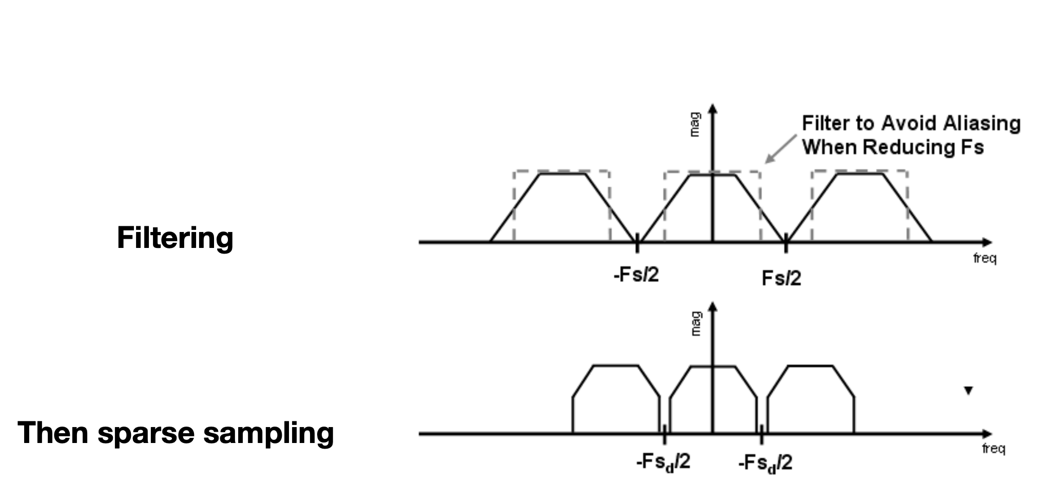
| 2. Anti-aliasing | Make frequency content “narrower” (filter out high frequencies before sampling) by blurring, then sample | Requires “filter first, then sample” |
Practical Pre-filtering: 1-Pixel-Wide Box Filter
How:
- Convolve $f(x,y)$ with a 1-pixel-wide box blur (low-pass).
- Then sample at each pixel center.
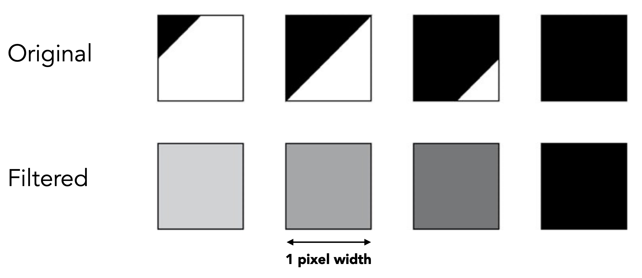
Key insight: when rasterizing a single triangle, the average value of $f(x,y) = inside(triangle, x, y)$ over the pixel area equals exactly the fraction of the pixel area covered by the triangle.
- 100% covered → pixel value 1 (solid color)
- 50% covered → pixel value 0.5 (intermediate color)
10 Common Anti-Aliasing Techniques
MSAA (Multisample Anti-Aliasing)
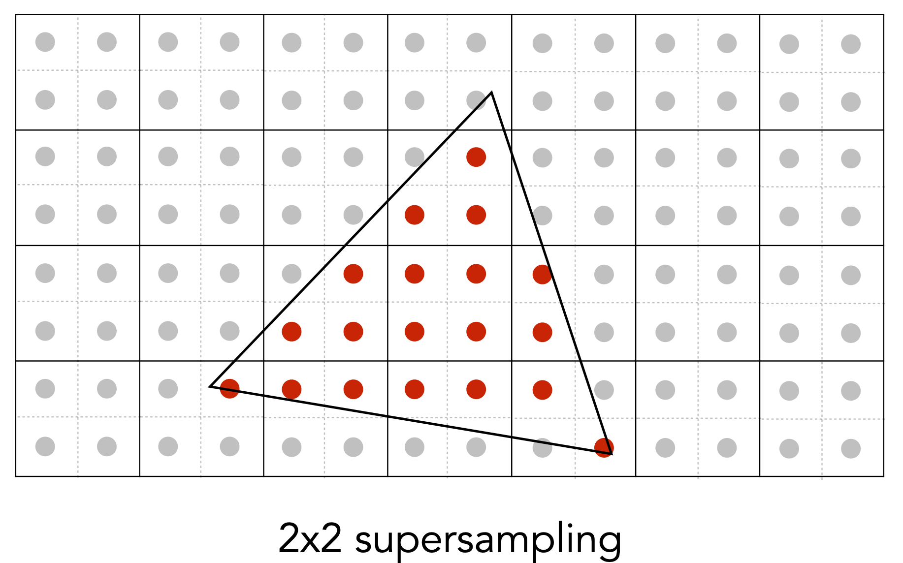
Note the distinction: “supersampling anti-aliasing” refers to SSAA (Super Sampling Anti-Aliasing), which subdivides each pixel into $N \times N$ sub-pixels, each of which is fully rendered independently (depth + shading) and then averaged — shading cost scales by ~$N^2$. MSAA (Multisample Anti-Aliasing) is an efficient optimization of SSAA: the sub-sample points only perform visibility (coverage) tests, not independent shading; the whole pixel is shaded once at its center, then blended weighted by coverage. Since computing exact coverage is hard, multiple sample points are used to approximate a 1-pixel box filter.
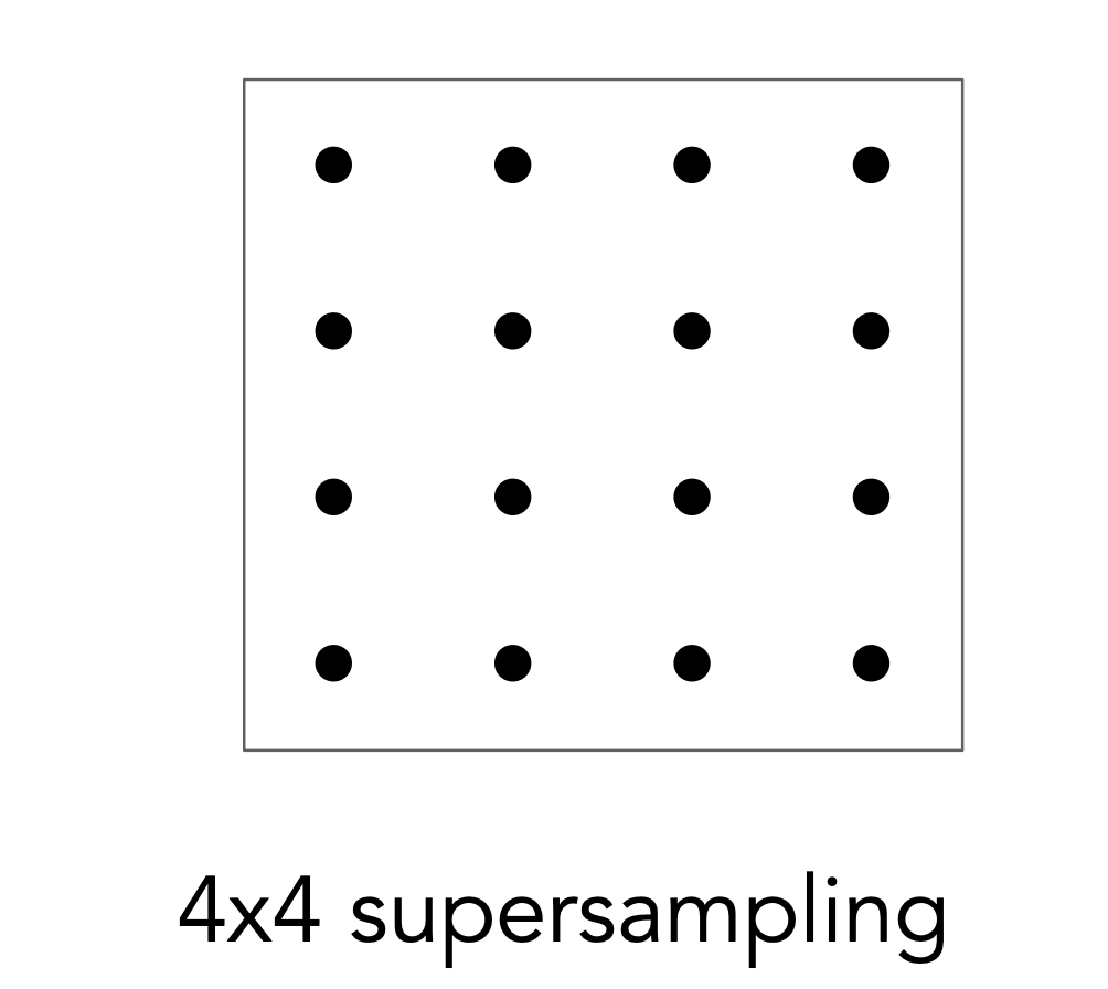
Steps (sub-samples only participate in coverage tests; shading is done once):
- Subdivide each pixel into $N \times N$ sub-sample points.
- Test each sub-sample point against the triangle (1 or 0) to obtain coverage.
- Shade once at the pixel center (or centroid), then weight-blend the color by coverage to get the pixel value.
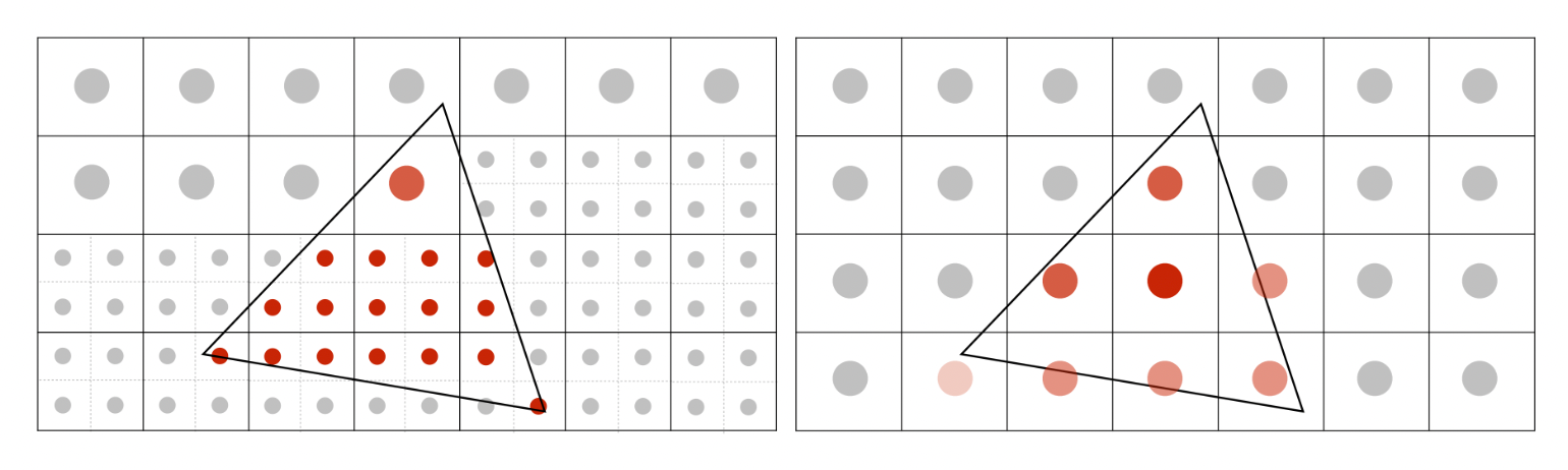
Result: edge pixels get intermediate values like 25% / 50% / 75% / 100%, showing smooth transitions.
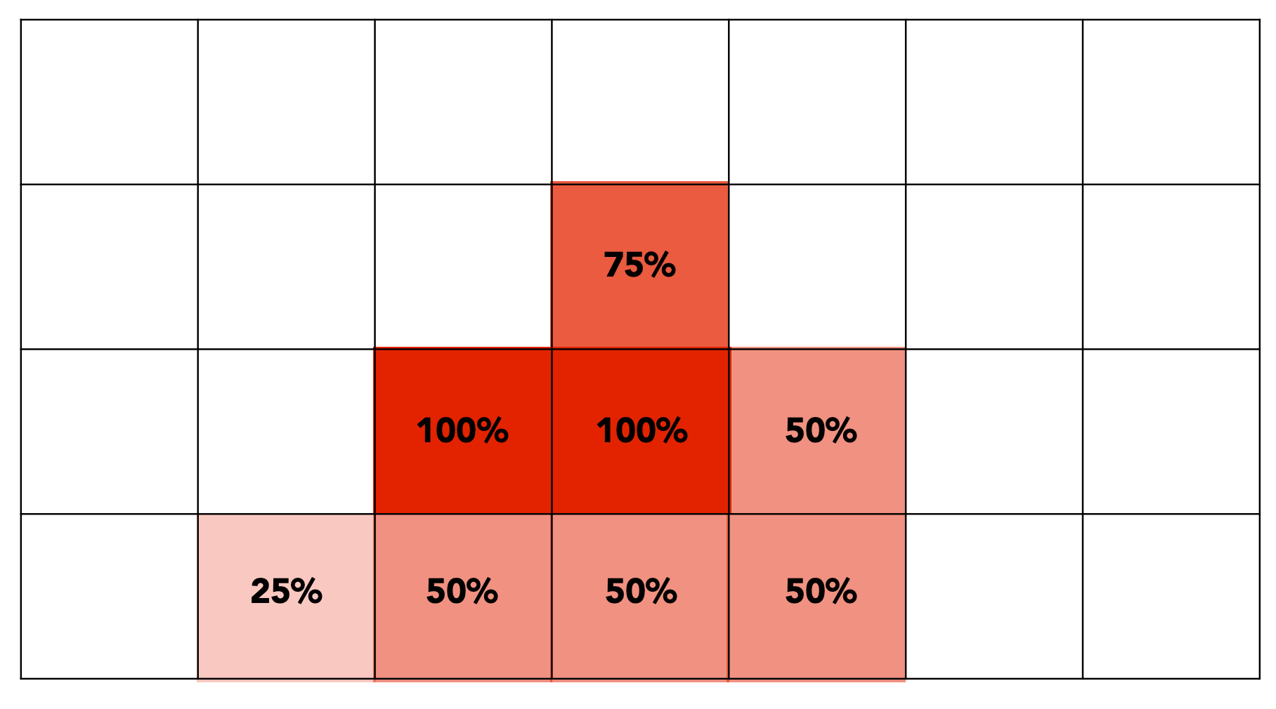
Pros: effective, reliably eliminates jaggies.
Cons: more sample points add extra coverage tests and color/depth storage overhead (stored per sample point in hardware); but shading runs only once, far cheaper than SSAA (the ~$N^2$ cost increase is characteristic of SSAA).
FXAA (Fast Approximate Anti-Aliasing)
Fast approximate anti-aliasing: a post-processing technique.
Principle:
- No extra sample points.
- After rendering, detect edges in the image.
- Smooth/blend pixels near the edges.
Pros: fast, low performance cost.
Cons: may lose detail.
TAA (Temporal Anti-Aliasing)
Temporal anti-aliasing: exploits information across frames.
Principle:
- In different frames, sample different positions within a pixel (jittered per frame).
- Blend results across frames (accumulate over time).
Pros: good quality, suits dynamic scenes, low per-frame cost.
Cons: may cause ghosting.
Super Resolution and DLSS
- Super Resolution / Super Sampling: reconstruct a high-resolution image from a low-resolution one; essentially still a “undersampling” problem.
- DLSS (Deep Learning Super Sampling): deep-learning supersampling — render at low resolution and use AI inference to output a high-resolution image; an important direction in recent real-time rendering.
11 Review Quiz
1. How do fovY, aspect ratio, and the near clip plane $l,r,b,t$ convert between each other?
Assuming a symmetric frustum ($l=-r$, $b=-t$), from the right triangle formed on the near clip plane:
$$ t = |n| \cdot \tan\frac{fovY}{2} \;\Rightarrow\; b = -t $$Then from aspect = width / height = r / t:
$$ r = t \cdot \text{aspect} \;\Rightarrow\; l = -r $$So given fovY, aspect, and near plane distance $n$, we can fully determine $l, r, b, t$.
2. Why is the viewport transformation independent of z? What determine its translation and scaling factors?
- Why independent of z: the viewport transformation maps the screen coordinates (x, y) of the canonical cube $[-1,1]^2$ to the display pixel range $[0, width] \times [0, height]$. Depth z was already handled in projection (kept for the depth buffer; it does not participate in screen imaging).
- Translation factors: $\frac{width}{2}$, $\frac{height}{2}$ — shift the scaled, origin-centered image to the screen center so the range becomes $[0, width]$, $[0, height]$.
- Scaling factors: $\frac{width}{2}$, $\frac{height}{2}$ — scale coordinates from $[-1,1]$ to $[0, width]$ / $[0, height]$ (factor = half the range span).
The third row of $M_{viewport}$ is $(0, 0, 1, 0)$, passing z through unchanged for later depth testing.
3. What is the principle behind the cross-product point-in-triangle test? Why does “same sign” mean inside?
For triangle ABC, traverse the three edges AB, BC, CA in a consistent orientation (CCW or CW) and compute the z component of the cross product of the edge vector and the “vertex → P” vector:
$$ z_k = \text{cross}(\text{edge}_k, \text{vertex}_k \to P).z $$- The sign of the cross-product z component tells whether P is on the left (>0) or right (<0) of that edge.
- If P is inside the triangle, it must lie on the same side of all three directed edges — all three z components have identical signs (all positive or all negative).
- If any z component differs in sign, P is outside that edge, hence outside the triangle.
“Same sign = inside” is a geometric consequence of convexity: a triangle, as a convex region, is equivalent to the intersection of “same-side” half-planes of its three directed edges.
4. Why does “filter first, then sample” remove jaggies while “sample first, then filter” only yields blurred jaggies?
- Filter first, then sample (correct): the original continuous signal $f(x,y)$ contains high frequencies (e.g. the step at a triangle edge). Low-pass filtering first (1-pixel box blur) removes frequencies beyond the sampling limit in advance, so the remaining frequencies satisfy the Nyquist condition and sampling produces no aliasing. Edge pixels naturally land on intermediate values between 0 and 1, giving smooth anti-aliased edges.
- Sample first, then filter (wrong): sampling the original high-frequency signal at an insufficient rate already aliases high frequencies into wrong low-frequency signals — the information is irrecoverably lost. Low-pass filtering such a discrete signal (containing spurious aliased frequencies) only blurs the false low-frequency content along with the true signal, producing an image that is still jagged but blurry — jaggies remain, and sharpness is lost.
Core: aliasing happens at the moment of sampling. High frequencies must be filtered out before sampling to prevent aliasing; filtering after sampling cannot “undo” aliasing that already occurred.
5. How do you understand “sampling = repeating frequency content” and “aliasing = mixing frequency content”?
- Sampling = repeating frequency content: in the frequency domain, uniform sampling is equivalent to multiplying the original spectrum by an impulse train (Dirac comb). By the convolution theorem, this corresponds to periodically copying the spectrum at integer multiples of the sampling frequency $f_s$, with copy spacing exactly $f_s$. Higher sampling rate → larger copy spacing.
- Aliasing = mixing frequency content: when the sampling rate is too low ($f_s$ too small), adjacent copies overlap; information originally at high frequencies is “folded” into the low-frequency region and becomes indistinguishable from genuine low frequencies — high frequency masquerades as low frequency, i.e. aliases. On images this shows as jaggies, Moiré, and other artifacts.
Essence of the Nyquist sampling theorem: to prevent copies from overlapping, the sampling rate must satisfy $f_s \geq 2 f_{\text{max}}$; otherwise high and low frequencies mix.
6. What are the principles, pros/cons, and use cases of MSAA, FXAA, TAA, and DLSS?
| Technique | Principle | Pros | Cons | Use cases |
|---|---|---|---|---|
| MSAA | Subdivide each pixel into $N \times N$ sub-samples, test each against inside(triangle), average by coverage, approximating a 1-pixel box pre-filter | Effective, clear principle, smooth geometry edges | Extra coverage tests and color/depth storage overhead per sample point, but shading runs only once — far cheaper than SSAA; does not fix shader/texture aliasing | Geometry-edge anti-aliasing, default AA in traditional engines |
| FXAA | Post-processing: detect edges after rendering, smooth/blend nearby pixels | Fast, cheap, independent of scene complexity | May lose detail, can blur high-contrast edges, does not solve temporal aliasing | Mobile, performance-limited platforms, quick approximate AA |
| TAA | Exploits frame-to-frame correlation: jittered sampling within each pixel per frame, accumulated over time, equivalent to “high sampling rate” | Low per-frame cost, better than MSAA, handles shader/transparent aliasing | Ghosting in dynamic scenes, relies on motion vectors, sensitive to fast motion | Mainstream in modern real-time engines (UE, Unity HDRP) |
| DLSS | Deep-learning supersampling: render below output resolution, neural network reconstructs high-res using history frames + motion vectors + input frame | Significant performance gain, sharper than traditional TAA, sometimes exceeds native rendering | Depends on AI hardware (Tensor Core), may produce artifacts, quality varies across versions (1/2/3) | RTX GPUs, AI-accelerated real-time rendering |
Comparison summary:
- MSAA truly adds sample points, addressing spatial-domain aliasing.
- FXAA / TAA both use “post-processing + information reuse”, compensating for insufficient samples via algorithms / historical frames.
- DLSS goes further with “AI priors”: instead of per-pixel operations, it learns an image-to-image mapping, becoming a new benchmark in super-resolution.
This is note 4 in the GAMES101 - Modern Computer Graphics study series.