- Instructor: Lingqi Yan | UCSB
- Bilibili: https://www.bilibili.com/video/BV1X7411F744
- Lectures covered: Lecture 17 (Materials and Appearances)
Note: the previous post (#7) drove all the way to path tracing and solved the rendering equation. This one turns around and stares at the one term in that equation that is “known” yet endlessly complicated — $f_r$, the BRDF. Materials, appearances, glossiness, Fresnel, microfacets: they all answer the same question. When light hits this surface, how much energy goes where? The advanced rendering topics of Lecture 18 (BDPT, MLT, photon mapping, VCM, plus non-surface models such as participating media and hair) get their own post.
1 Materials and Appearances
Take one mesh and assign different materials to different parts, and the rendering changes completely: glazed ceramic shows a partial specular highlight, clay is diffuse, and the coffee on top is textured.
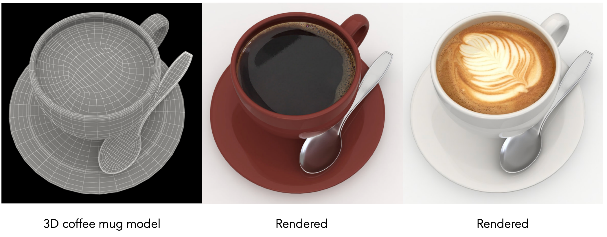
In graphics, a material is a BRDF. Different BRDFs define different material appearances — the BRDF decides how light gets reflected.
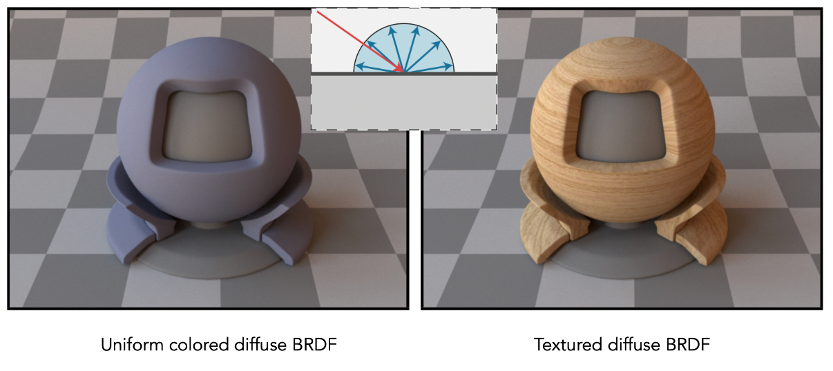
The family of materials we walk through looks roughly like this:
| Material type | BRDF characteristics | Typical appearance |
|---|---|---|
| Diffuse | Reflects uniformly in every direction, $f_r = \rho/\pi$ | Clay, paper, rubber |
| Glossy | Reflection concentrated in a small cone around the specular direction | Copper, aluminium and other metals |
| Ideal specular reflection / refraction | Dirac $\delta$, light leaves along a single direction | Mirrors, glass, water |
| Microfacet | Determined by the distribution of microfacet normals | Brushed metal, leather, car paint |
2 Diffuse / Lambertian Material
Light is reflected uniformly into all directions.
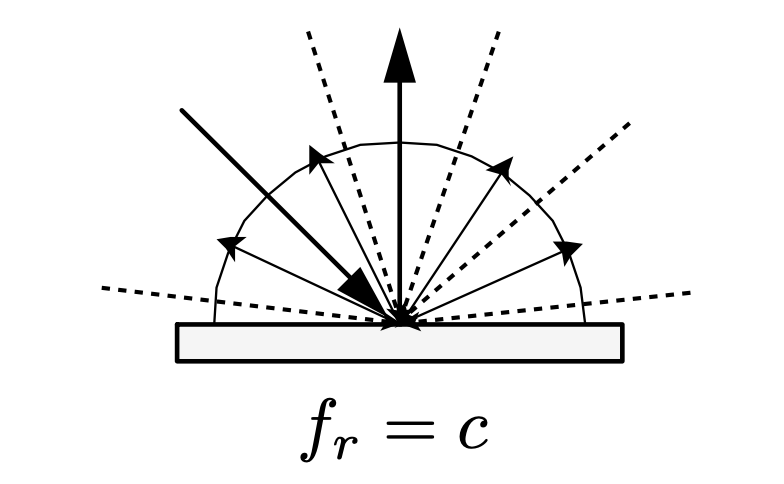
BRDF:
$$ f_r = \frac{\rho}{\pi} $$where $\rho$ is the albedo — the colour of the surface.
Derivation: assume the incoming light is uniform ($L_i$ constant). By energy conservation (the point emits no light and absorbs none, so whatever it receives it must reflect):
$$ L_o(\omega_o) = \int_{H^2} f_r \, L_i \cos\theta_i \, d\omega_i = f_r \, L_i \int_{H^2} \cos\theta_i \, d\omega_i = \pi f_r L_i $$Since $\int_{H^2} \cos\theta_i \, d\omega_i = \pi$ over the hemisphere, if $L_o = L_i$ (perfect reflection, no absorption at all) then $f_r = \frac{1}{\pi}$. Multiply by the albedo $\rho$ and you get the diffuse BRDF.
3 Glossy Material
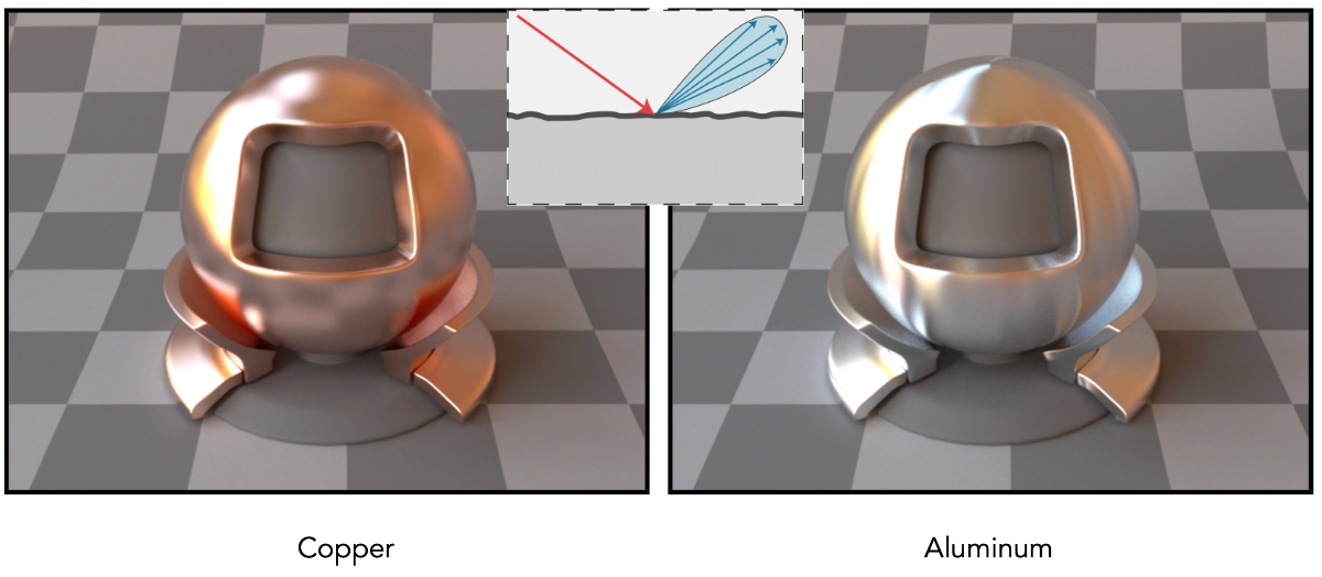
Somewhere between diffuse and a perfect mirror: reflected light concentrates in a small range around the specular direction instead of spreading out uniformly or collapsing to a single ray. Copper and aluminium surfaces behave like this.
4 Ideal Reflective / Refractive Material
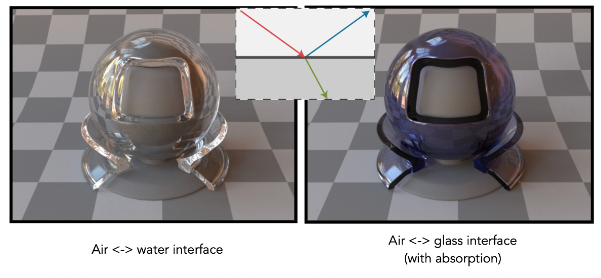
When light travels from one medium (say air) towards another (say glass), the change in propagation speed splits it: part is specularly reflected, part enters the new medium and bends.
Such materials handle reflection and refraction together, which is why they are also called a BSDF (Bidirectional Scattering Distribution Function).
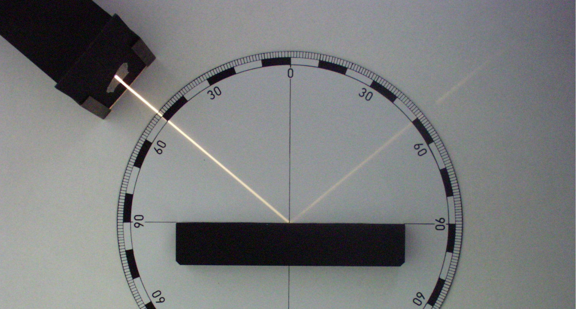
Perfect Specular Reflection
Azimuth is the horizontal angle measured from a reference direction (usually due north) clockwise to the target direction.
Angle of incidence equals angle of reflection: $\theta_i = \theta_o = \theta$
Azimuth relation: $\phi_o = (\phi_i + \pi) \mod 2\pi$
Computing the reflected direction:
$$ \omega_o + \omega_i = 2 \cos \theta \vec{n} = 2(\omega_i \cdot \vec{n})\vec{n} $$$$ \omega_o = -\omega_i + 2(\omega_i \cdot \vec{n})\vec{n} $$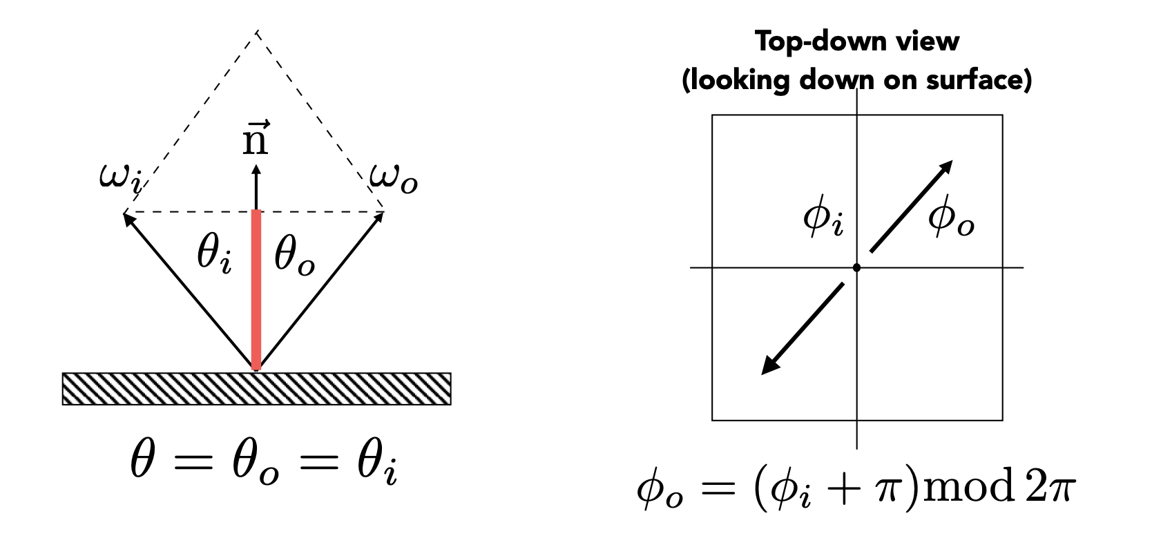
The BRDF of perfect specular reflection can be written as a Dirac $\delta$ — it is non-zero only along the mirrored direction, and zero everywhere else.
Specular Refraction
Light can also pass through the surface. Entering a new medium makes it refract.
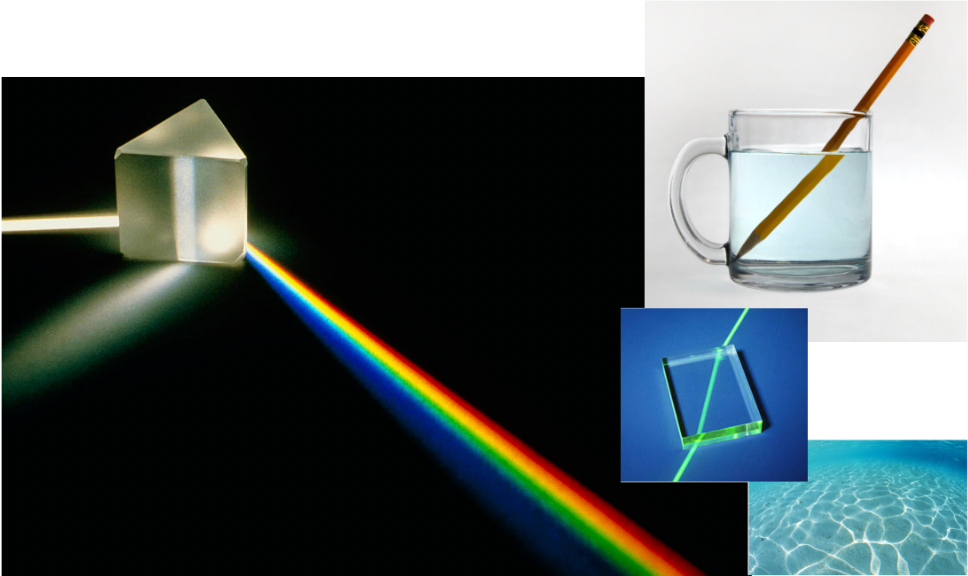
Snell’s Law: the refracted angle depends on the index of refraction (IOR) of the media on both sides. Different materials have different IORs.
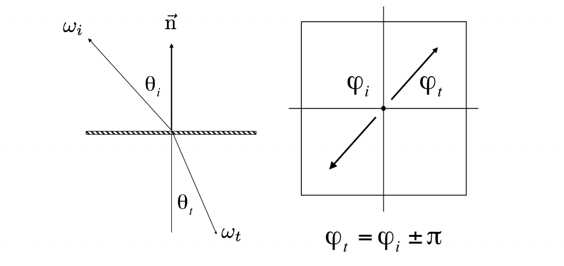
where $\eta_i$ and $\eta_t$ are the IORs of the incident and transmitting media.
Common indices of refraction:
| Medium | IOR |
|---|---|
| Vacuum | 1.0 |
| Air (sea level) | 1.00029 |
| Water (20C) | 1.333 |
| Glass | 1.5 - 1.6 |
| Diamond | 2.42 |
Computing the refracted angle:
$$ \cos\theta_t = \sqrt{1 - \sin^2\theta_t} = \sqrt{1 - \left(\frac{\eta_i}{\eta_t}\right)^2 \sin^2\theta_i} = \sqrt{1 - \left(\frac{\eta_i}{\eta_t}\right)^2 (1 - \cos^2\theta_i)} $$Total Internal Reflection: when light travels from a denser to a rarer medium ($\eta_i / \eta_t > 1$) at a sufficiently large angle of incidence:
$$ 1 - \left(\frac{\eta_i}{\eta_t}\right)^2 (1 - \cos^2\theta_i) < 0 $$The value under the square root goes negative, so $\cos\theta_t$ has no real solution and refraction simply does not exist. Look at the condition: $1 - \cos^2\theta_i$ lies in $[0, 1]$, so only $\frac{\eta_i}{\eta_t} > 1$ (denser to rarer) can make the radicand negative. The light cannot escape and is entirely reflected back into the original medium.
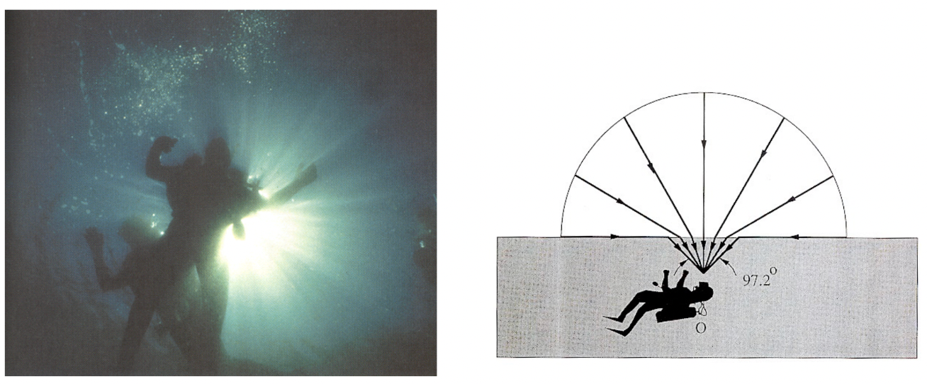
Snell’s Window / Circle: the visible consequence of total internal reflection — looking up at the water surface from below, you only see the world above through a circular patch overhead; outside that circle, total internal reflection shows you a mirror image of the water below.
5 The Fresnel Term
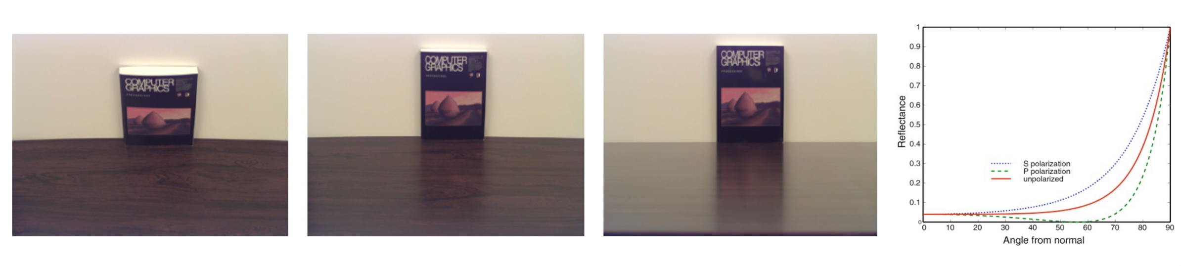
The phenomenon: reflectance depends on the angle of incidence — the more grazing the view, the stronger the reflection. That is why distant water surfaces and tabletops always look “reflective”.
| Type | Notes |
|---|---|
| Dielectric | Glass, water — reflectance rises sharply at grazing angles |
| Conductor | Metals — reflectance is high at all angles |
The exact formulas (accounting for polarisation; for reference only):
$$ R_{\mathrm{s}} = \left| \frac{n_1 \cos \theta_{\mathrm{i}} - n_2 \cos \theta_{\mathrm{t}}}{n_1 \cos \theta_{\mathrm{i}} + n_2 \cos \theta_{\mathrm{t}}} \right|^2 = \left| \frac{n_1 \cos \theta_{\mathrm{i}} - n_2 \sqrt{1 - \left( \frac{n_1}{n_2} \sin \theta_{\mathrm{i}} \right)^2}}{n_1 \cos \theta_{\mathrm{i}} + n_2 \sqrt{1 - \left( \frac{n_1}{n_2} \sin \theta_{\mathrm{i}} \right)^2}} \right|^2, $$$$ R_{\mathrm{p}} = \left| \frac{n_1 \cos \theta_{\mathrm{t}} - n_2 \cos \theta_{\mathrm{i}}}{n_1 \cos \theta_{\mathrm{t}} + n_2 \cos \theta_{\mathrm{i}}} \right|^2 = \left| \frac{n_1 \sqrt{1 - \left( \frac{n_1}{n_2} \sin \theta_{\mathrm{i}} \right)^2} - n_2 \cos \theta_{\mathrm{i}}}{n_1 \sqrt{1 - \left( \frac{n_1}{n_2} \sin \theta_{\mathrm{i}} \right)^2} + n_2 \cos \theta_{\mathrm{i}}} \right|^2. $$$$ R_{eff} = \frac{1}{2}(R_s + R_p) $$The Schlick approximation (faster, and what renderers actually use):
$$ R(\theta) = R_0 + (1 - R_0)(1 - \cos\theta)^5 $$- $R(\theta)$: reflectance at angle of incidence $\theta$
- $R_0$: the base reflectance at normal incidence ($\theta = 0$)
- $\theta$: the angle of incidence (between ray and normal)
- $\cos\theta$: the dot product of incident direction and normal (for unit vectors)
where $R_0$ follows from the two IORs:
$$ R_0 = \left(\frac{n_1 - n_2}{n_1 + n_2}\right)^2 $$// cosTheta = dot(normal, viewDir), both unit vectors
float R0 = pow((n1 - n2) / (n1 + n2), 2.0);
float fresnel = R0 + (1.0 - R0) * pow(1.0 - cosTheta, 5.0);
The Schlick approximation uses two terms, $R_0$ and $(1 - \cos\theta)^5$, to turn the complicated Fresnel equations into a fast interpolation: it returns $R_0$ at normal incidence, approaches 1 at grazing angles, and transitions smoothly in between.
6 Microfacet Material
The Earth is not a smooth sphere — it has mountains and basins — yet photographs from space still show a specular highlight.
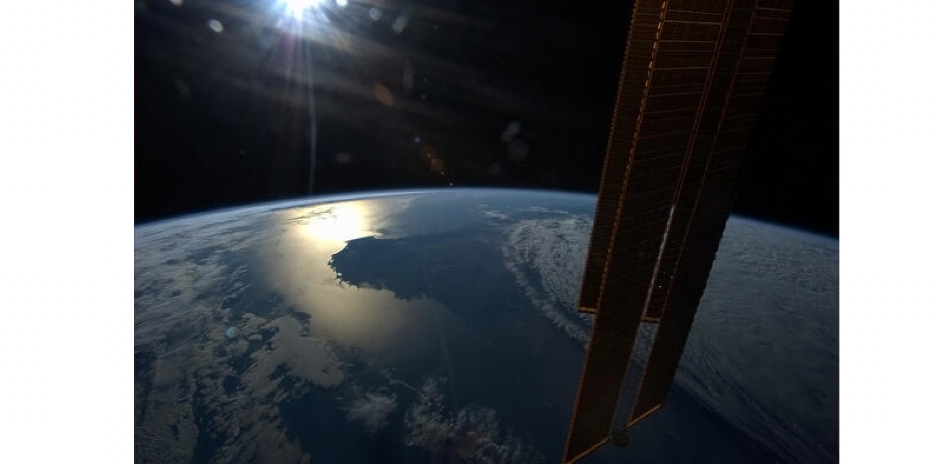
Microfacet theory
- Macroscale: the surface is flat and rough
- Microscale: the surface is bumpy, and each microfacet behaves like a tiny mirror
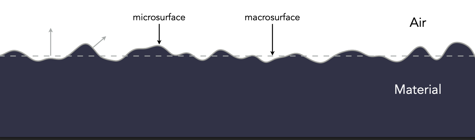
The microfacet BRDF
The key is the distribution of microfacet normals.
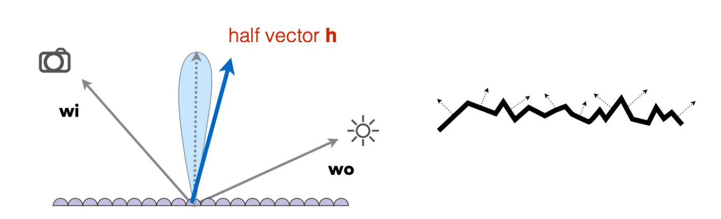
- Normals concentrated $\Rightarrow$ glossy
- Normals spread out $\Rightarrow$ diffuse
| Term | Meaning |
|---|---|
| $F(i, h)$ | Fresnel term: how much light is reflected |
| $G(i, o, h)$ | Shadowing-masking term: occlusion between microfacets |
| $D(h)$ | Normal distribution function (NDF): distribution of microfacet normals |
| $h$ | Half vector: the direction halfway between $\omega_i$ and $\omega_o$ |
Microfacet materials show up everywhere: motorcycle dashboards, rough cushions, smooth leather, near-mirror metals, wooden furniture.
7 Isotropic and Anisotropic Materials
In materials and rendering, isotropic and anisotropic describe whether a surface’s properties depend on direction.
The one-line difference: an isotropic material’s reflection looks the same as you rotate the object; an anisotropic material’s reflection stretches and deforms with direction.
| Type | Notes | BRDF property | Examples |
|---|---|---|---|
| Isotropic | Microfacet normals have no directional preference | $f_r(\theta_i, \phi_i; \theta_r, \phi_r) = f_r(\theta_i, \theta_r, \phi_r - \phi_i)$ | Most materials |
| Anisotropic | Microfacets have directional structure | $f_r(\theta_i, \phi_i; \theta_r, \phi_r) \neq f_r(\theta_i, \theta_r, \phi_r - \phi_i)$ | Brushed metal, nylon, velvet |
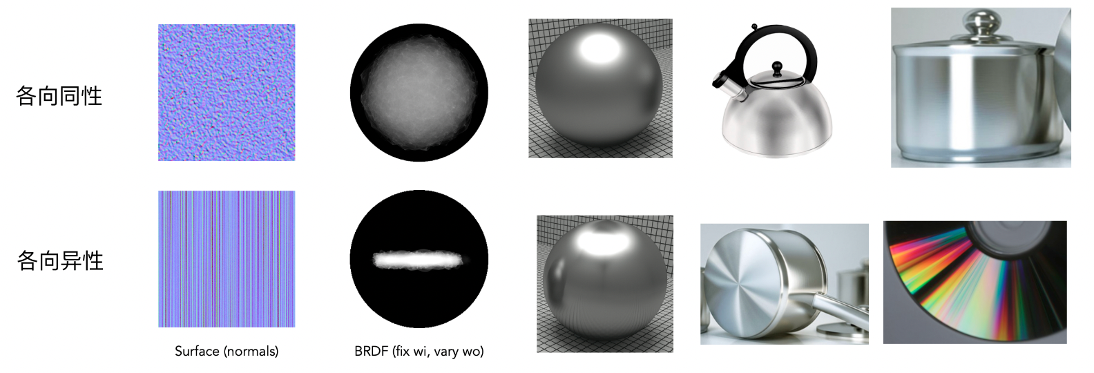
An anisotropic material’s reflection varies with azimuth because of directional microstructure on the surface — the grain direction of brushed metal, for instance.
8 Properties of BRDFs
| Property | Formula | Notes |
|---|---|---|
| Non-negativity | $f_r(\omega_i \to \omega_r) \geq 0$ | Reflected energy cannot be negative — the most basic physical constraint |
| Linearity | $L_r(\omega_r) = \int_{\Omega} f_r(\omega_i \to \omega_r) \, L_i(\omega_i) \cos\theta_i \, d\omega_i$ | Contributions from multiple lights or multiple BRDFs add linearly — the basis for accumulating lights separately in a renderer |
| Reciprocity (reversibility) | $f_r(\omega_i \to \omega_r) = f_r(\omega_r \to \omega_i)$ | Swapping incident and outgoing directions leaves the BRDF unchanged, guaranteed by the Helmholtz reciprocity principle |
| Energy conservation | $\forall \omega_r,\ \int_{H^2} f_r(\omega_i \to \omega_r) \cos\theta_r \, d\omega_r \leq 1$ | Total reflected energy never exceeds incident energy. Equal to 1 means no absorption; less than 1 means some loss |
| Isotropy | $f_r(\theta_i, \phi_i; \theta_r, \phi_r) = f_r(\theta_i, \theta_r, \phi_r - \phi_i)$ | Rotating the whole scene about the normal leaves the BRDF unchanged; it depends only on the two polar angles and the azimuth difference |
| Anisotropy | $f_r = f_r(\omega_i, \omega_r, \mathbf{t})$ | Additionally depends on the surface tangent $\mathbf{t}$; rotation changes the reflection, as with brushed metal or optical discs |
| Symmetry | $f_r(\omega_i \to \omega_r) = f_r(\omega_r \to \omega_i)$ and $\int f_r \cos\theta \, d\omega \leq 1$ | Satisfying both reciprocity and energy conservation is the basic requirement for a physically correct BRDF |
| No self-emission | $f_r$ describes reflection only | Emission is a separate term and is not part of the BRDF |
A BRDF must satisfy three basic physical constraints — non-negativity, reciprocity and energy conservation. Beyond that it can be classified as isotropic or anisotropic, and it is linear.
9 BRDF Measurement
A BRDF is a theoretical model, but real materials reflect light in very complicated ways:
- The microstructure differs wildly from material to material
- The same material behaves completely differently at different angles
- Theoretical models (Cook-Torrance, for instance) are only approximations whose parameters need real data to be calibrated
So trustworthy BRDF data has to come from actual measurement.
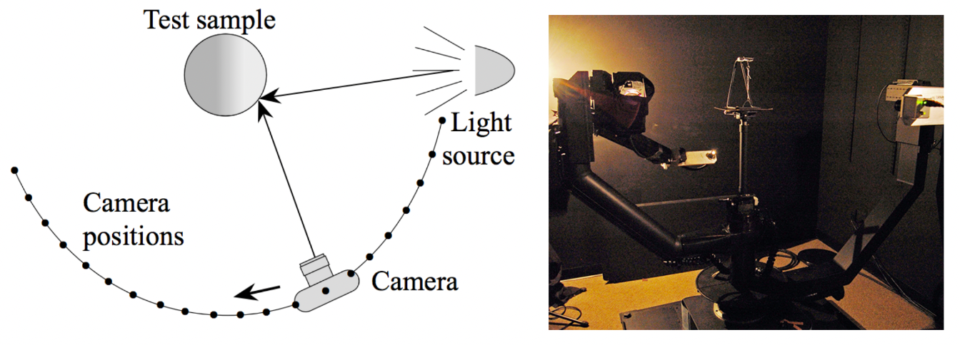
Motivation: skip developing and deriving a model, and render directly with real material data.
Method (using a gonioreflectometer):
for each outgoing direction wo:
    move the light source to illuminate the surface from wo
    for each incident direction wi:
        move the sensor to direction wi
        measure the incident radiance
Efficiency optimisations:
- For isotropic surfaces, the dimensionality drops from 4D to 3D
- Reciprocity halves the number of measurements
- Cleverer optical system design
Image-based measurement: Marschner et al. 1999 replaced point-by-point mechanical measurement with a camera.
Challenges in measurement:
- Accurate measurement at grazing angles (important because of the Fresnel effect)
- High-frequency specular peaks need dense enough sampling to capture
- Retro-reflection
- Spatially varying reflectance
Representing measured data: desirable properties are compactness, faithful reproduction of the measurements, efficient evaluation for arbitrary direction pairs, and suitability for importance sampling. A common choice is tabular representation: store regularly sampled values over $(\theta_i, \theta_o, |\phi_i - \phi_o|)$ (reparameterising when needed to match specular peaks better). Storage requirements are heavy — the MERL BRDF database [Matusik et al. 2004], for example, holds 90 × 90 × 180 sets of measurements.
Summary
This chapter is the gateway to the “materials” side, taking apart the known term $f_r$ in the rendering equation:
| Topic | Core content |
|---|---|
| A material is a BRDF | Different BRDFs define different appearances; in graphics, a material is a BRDF |
| Diffuse material | Energy conservation gives $f_r = \rho/\pi$, where $\rho$ is the albedo (colour) |
| Glossy material | Reflection concentrates near the specular direction — typical of copper and aluminium |
| Perfect specular reflection | $\theta_i = \theta_o$, $\omega_o = -\omega_i + 2(\omega_i \cdot \vec{n})\vec{n}$, BRDF is a Dirac $\delta$ |
| Specular refraction | Snell’s law $\eta_i \sin\theta_i = \eta_t \sin\theta_t$; total internal reflection and Snell’s window |
| Fresnel term | Reflectance rises with angle of incidence; Schlick approximation $R = R_0 + (1-R_0)(1-\cos\theta)^5$ |
| Microfacet material | $f = FGD / (4(n\cdot i)(n\cdot o))$; the normal distribution $D$ decides glossy vs diffuse |
| Isotropic / anisotropic | Whether reflection varies with azimuth depends on whether the microstructure is directional |
| Properties of BRDFs | Non-negativity, reciprocity, energy conservation — plus linearity and (an)isotropy |
| BRDF measurement | Gonioreflectometers and image-based capture; the MERL database is a standard source |
This post is note #8 in the GAMES101 - Modern Computer Graphics learning series.