- Instructor: Lingqi Yan | UCSB
- Bilibili: https://www.bilibili.com/video/BV1X7411F744
- Lectures covered: Lecture 20 (Light Field / Lumigraph, Color and Perception)
Note: these are two topics that step outside geometry. The light field asks how much information a scene actually carries visually; colour asks why that information turns into colour once it enters the human eye. They look unrelated but point at the same conclusion: the “image” and the “colour” we perceive are only low-dimensional projections of the physical world onto human senses — the light field squeezes the 7D plenoptic function down to 4D, and colour squeezes an infinite-dimensional spectrum down to 3D. It is precisely because this compression exists that image capture and colour reproduction are possible at all.
1 Light Field / Lumigraph
What we see
Looking out from a single viewpoint, the 3D world is flattened into a 2D image.
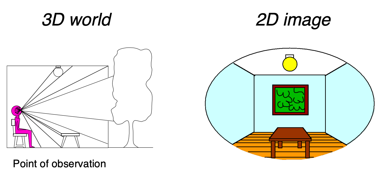
This also explains why a “painted backdrop” can fool the eye — as long as you look from one specific viewpoint, a 2D backdrop and a real 3D scene can produce exactly the same image.
The plenoptic function
The question: what is the set of everything we can see?
The answer: the plenoptic function (Adelson & Bergen).
The plenoptic function is the more complete, higher-dimensional generalization of the light field, introduced by Adelson and Bergen in 1991. It describes the complete set of rays at any position in space, in any direction, at any wavelength, at any instant.
Let us start from “a person standing still”, parameterize everything they can see, and then gradually relax the restrictions:
| Level | Expression | Description |
|---|---|---|
| Greyscale snapshot | $P(\theta, \varphi)$ | Light intensity: single viewpoint, single instant, averaged over the visible spectrum |
| Colour snapshot | $P(\theta, \varphi, \lambda)$ | Light intensity: single viewpoint, single instant, as a function of wavelength |
| Movie | $P(\theta, \varphi, \lambda, t)$ | Light intensity: single viewpoint, varying over time, as a function of wavelength |
| Holographic movie | $P(\theta, \varphi, \lambda, t, V_X, V_Y, V_Z)$ | Light intensity: any viewpoint, varying over time, as a function of wavelength |
The meaning of each dimension:
| Dimension | Symbol | Meaning |
|---|---|---|
| Horizontal direction | $\theta$ | Direction angle of the ray in the horizontal plane |
| Vertical direction | $\varphi$ | Direction angle of the ray in the vertical plane |
| Wavelength | $\lambda$ | Colour / spectrum of the light |
| Time | $t$ | How the light changes over time |
| Spatial position | $(V_x, V_y, V_z)$ | 3D coordinates of the viewpoint in space |
The plenoptic function contains every photograph, every movie and everything anyone has ever seen — it captures our visual reality completely. That is quite something for a single function.
From 7D to 5D: rays
Set time and colour aside for the moment and keep only space and direction:
$$ P(\theta, \varphi, V_X, V_Y, V_Z) $$This is 5D: 3D position + 2D direction.
From 5D to 4D: ray reuse
The key observation: in a vacuum (a non-dispersive medium), the intensity of light stays constant along an infinite straight line.
So every point along one ray shares the same value, and the position dimension can be dropped:
4D = 2D direction + 2D position
Outside the convex hull of the scene, we only need to record values on the plenoptic surface.
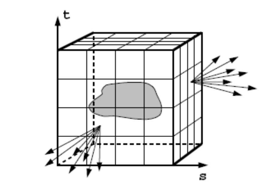
Once you have the 4D light field you can synthesize novel views — not by reconstructing geometry, but by direct table lookup and interpolation.
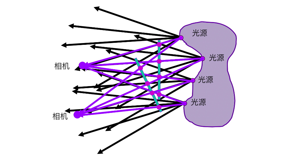
A light field = recording the position and direction of every ray. Compared with an ordinary photograph it retains the extra direction information, so it allows refocusing, depth-of-field adjustment and viewpoint changes after the fact; the price is resolution, data volume and compute cost. It is the key intermediate layer between ordinary imaging and the full plenoptic function.
How a Lumigraph / light field is organized
Outside the convex hull of the scene, space falls into two categories: empty and stuff. Light travels in straight lines with constant intensity through the “empty” regions, so recording them is very economical.
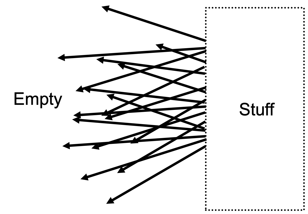
Two-plane parameterization: describe a ray with two parallel planes.
| Plane | Parameters | Meaning |
|---|---|---|
| First plane | $(s, t)$ | 2D position |
| Second plane | $(u, v)$ | 2D direction |
A ray is uniquely determined by the four coordinates $(s, t, u, v)$ at which it crosses the two planes.
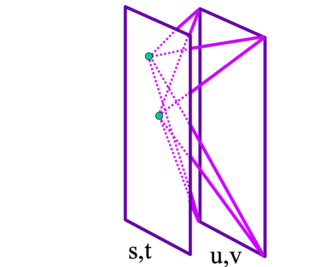
The key operation: fix $(s, t)$ and vary $(u, v)$ to obtain one image.
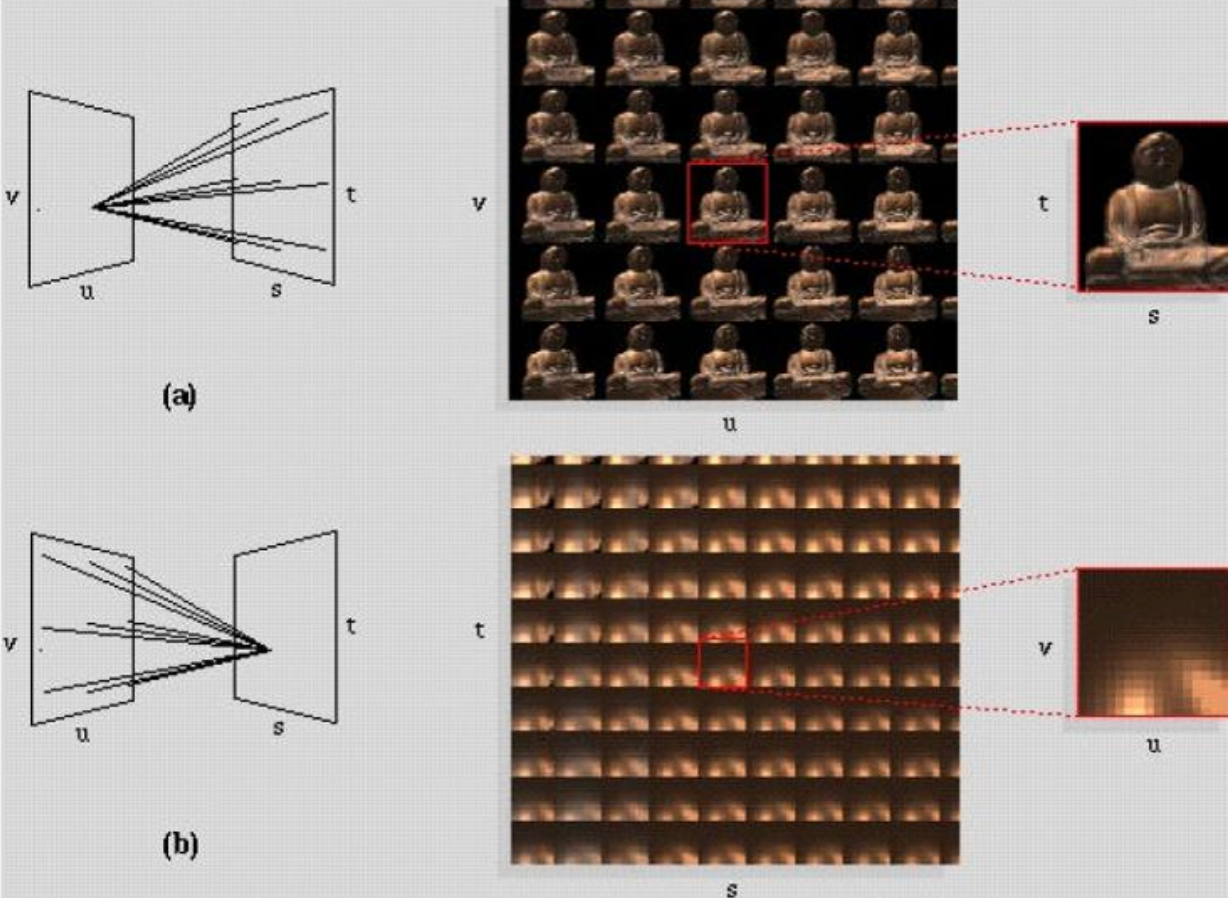
How light fields are captured
| Method | Description |
|---|---|
| Camera array | Stanford’s multi-camera array: a row of real cameras shoot simultaneously, each camera corresponding to one $(s,t)$ |
| Integral imaging (fly’s eye lenslets) | Spatially multiplexed light field capture with a microlens array (lenslets), proposed by Lippmann in 1908 |
The price of integral imaging: it imposes a fixed trade-off between spatial resolution and angular resolution — the same sensor has to record both spatial and directional information, and the two inevitably eat into each other.
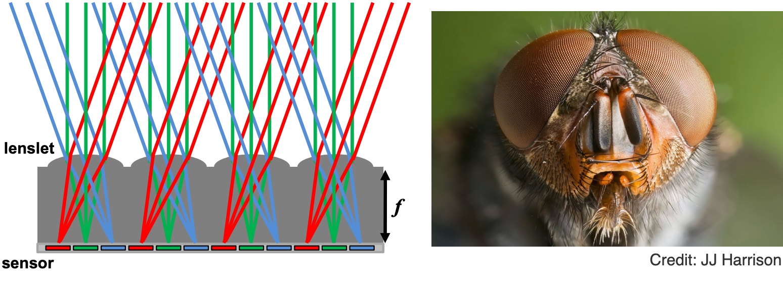
The light field camera
A light field camera records the position and direction of rays using a microlens array, enabling focus-after-shooting, depth estimation and multi-view synthesis. Its advantages are post-hoc flexibility and rich information; its drawbacks are low spatial resolution, large data volume and heavy computation. It is an important tool for computational photography and image-based rendering.
Lytro is the most famous light field camera product, founded by Professor Ren Ng at UC Berkeley, and its core is the microlens design.
Its most important feature: computational refocusing — after taking the picture you can still virtually change the focal length, the aperture size and so on.
How should we think about it?
- In a conventional camera, each pixel (one irradiance value) becomes, in a light field camera, a block of pixels (a set of radiance values)
- A block of pixels records light from the same spatial location in different directions
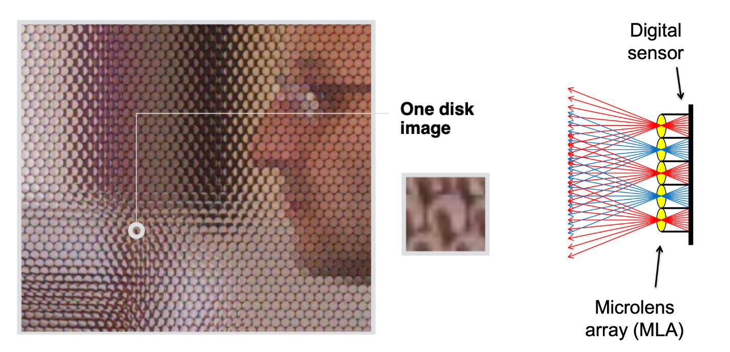
How do you get an “ordinary” photograph out of a light field photograph?
- The simplest case: always take the pixel at the bottom of each block
- Then take the middle one, then the top one
- This is essentially “moving the camera around”
Computational / digital refocusing uses the same idea: change the focal length visually, and pick the corresponding ray directions for the refocused image.
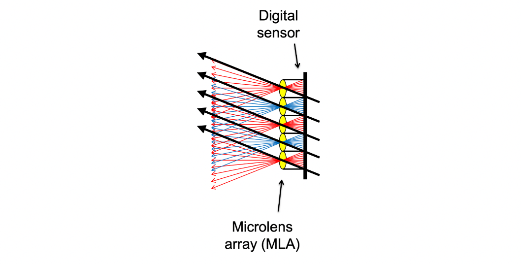
Problems with light field cameras
| Problem | Cause |
|---|---|
| Insufficient spatial resolution | The same piece of film carries both spatial and directional information |
| High cost | The microlens designation is extremely fine and complex |
Computer graphics is all about trade-offs. The light field camera trades spatial resolution for the freedom to “shoot first, focus later”.
2 The Physical Basis of Color
The basic composition of light
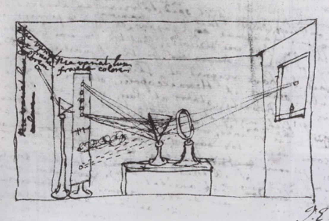
Newton used a prism to prove that sunlight can be split into a rainbow.
And the split light cannot be split any further by a second prism — which shows that each colour in the rainbow is already “elementary”.
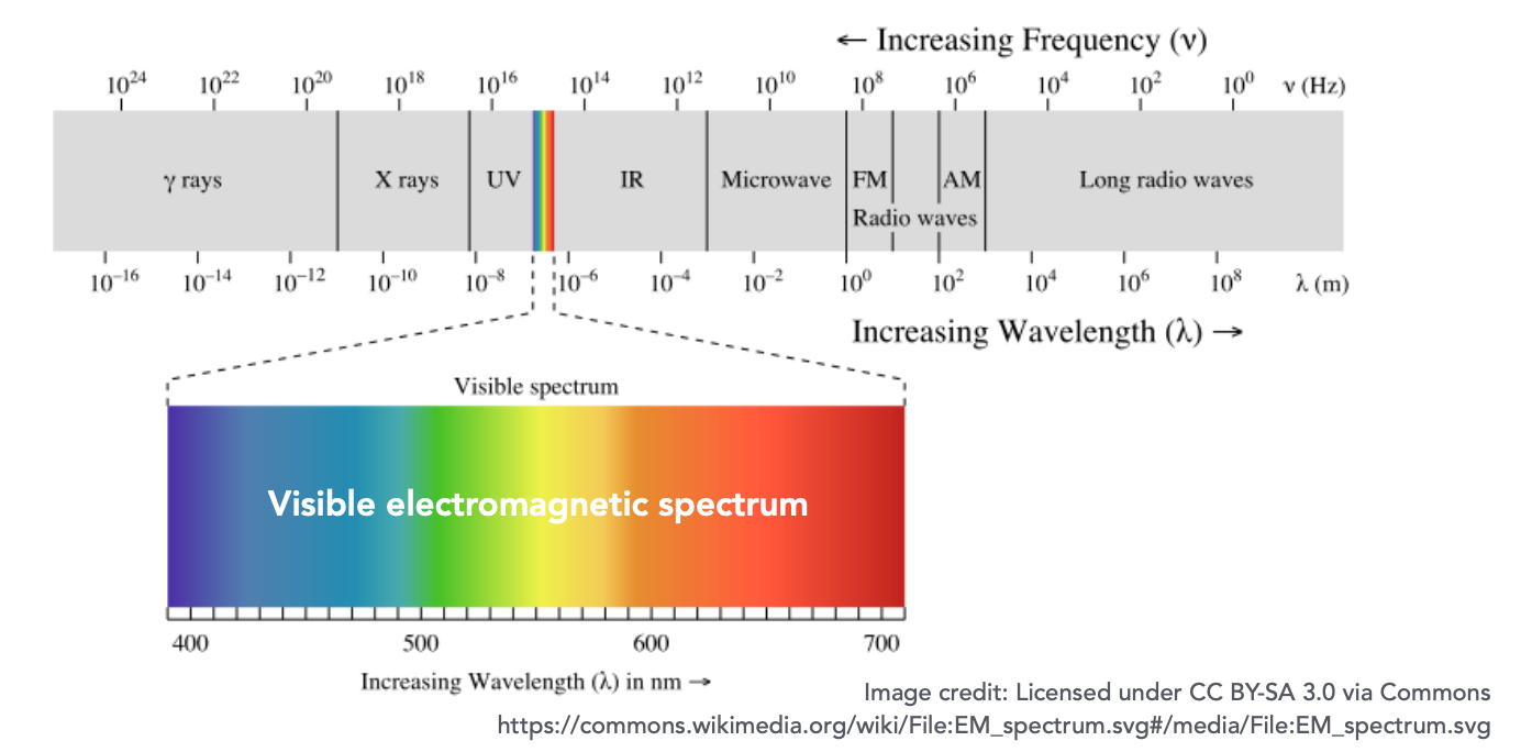
The visible spectrum
Light is electromagnetic radiation — oscillations at different frequencies (wavelengths).
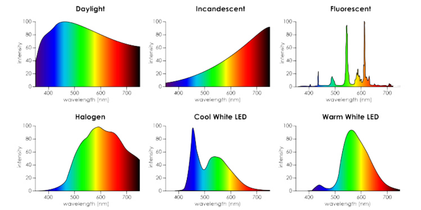
Spectral power distribution (SPD)
The spectral power distribution describes the power a light source radiates per unit wavelength interval — that is, the physical quantity “how much energy at which wavelength”.
A notable property when measuring light: how much light exists at each wavelength.
| Property | Description |
|---|---|
| Units | Radiometric units per nanometre (e.g. watts / nm), or dimensionless |
| Common practice | Use “relative units”, scaled to the maximum wavelength; convenient for comparing across wavelengths when absolute units do not matter |
Daylight SPDs differ from one another
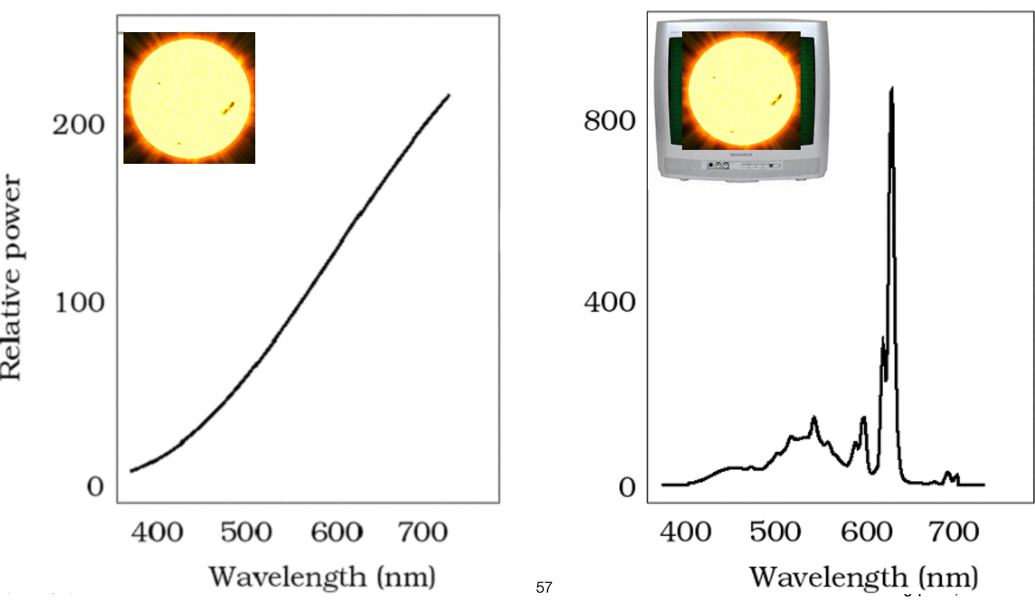
The SPD differs noticeably between conditions such as blue sky and the solar disc.
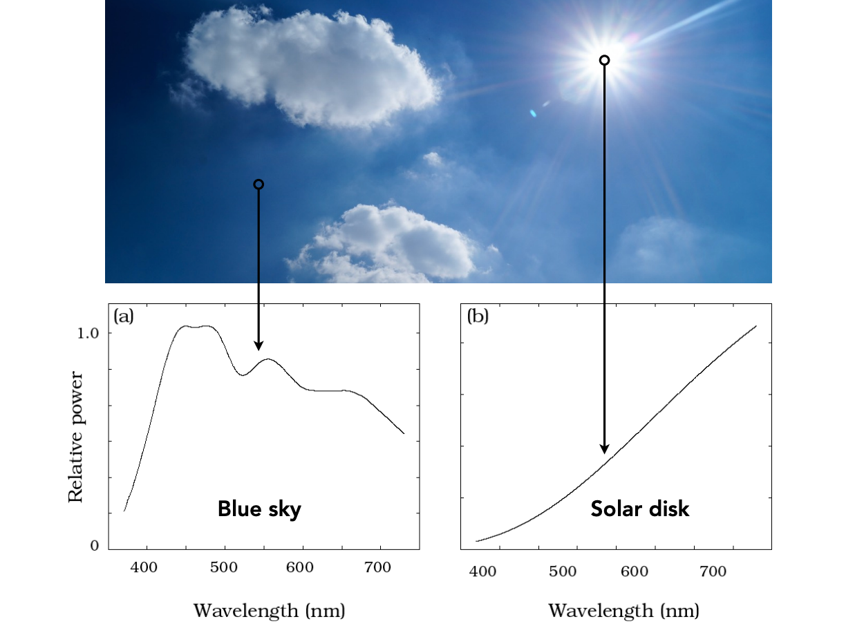
The SPD of a light source
The SPD describes the distribution of energy by wavelength — the most complete way to characterize a light source.
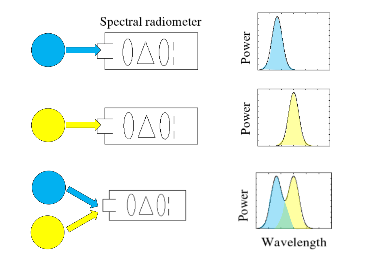
The linearity of SPDs
SPDs add linearly: when several light sources illuminate at once, the total SPD is the sum of the individual SPDs. This is the physical basis for “compute each light separately and add” in rendering.
What is colour?
Colour is a phenomenon of human perception; it is not a general property of light.
Light of different wavelengths is not “colour”.
3 The Biological Basis of Color
Anatomy of the human eye
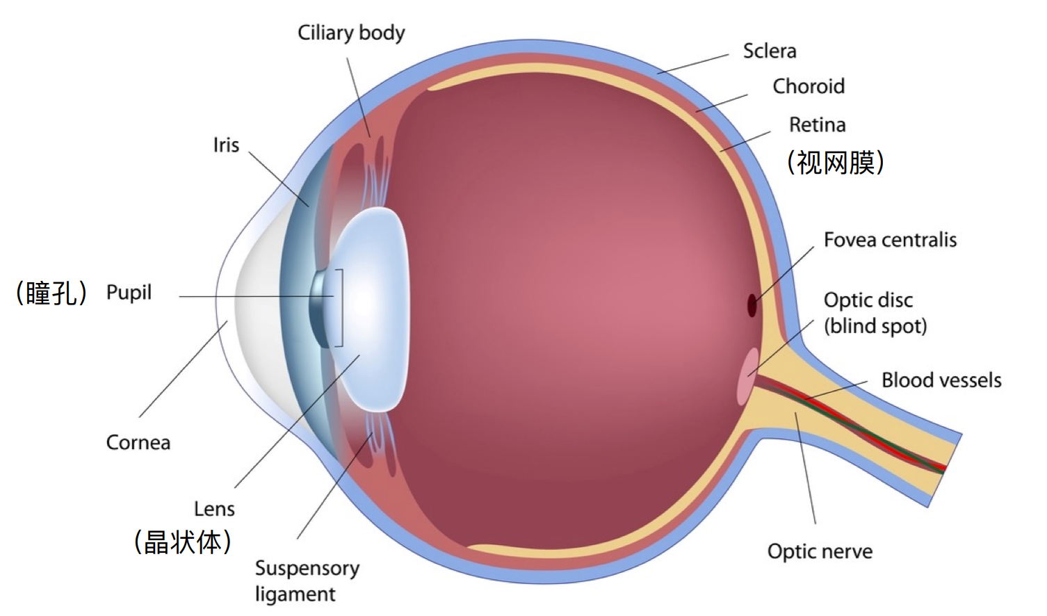
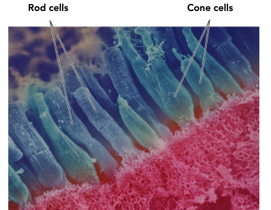
Retinal photoreceptors: rods and cones
| Type | Operating conditions | Count | Function |
|---|---|---|---|
| Rods | Very low illumination (scotopic vision), such as faint moonlight | About 120 million | Perceive only greyscale, no colour |
| Cones | Typical illumination (photopic vision) | About 6–7 million | Three types, each with a different spectral sensitivity, providing the sensation of colour |
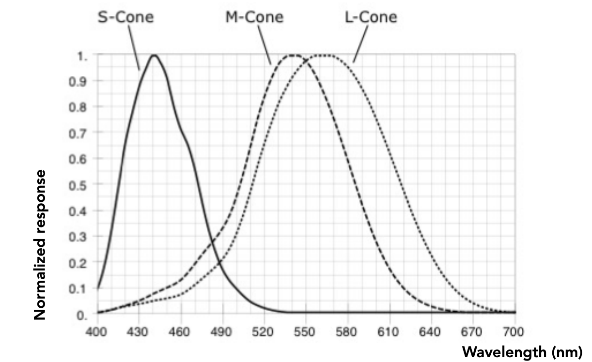
The spectral response of the three cone types
The three cone types S, M and L correspond to peak responses at short, medium and long wavelengths respectively.
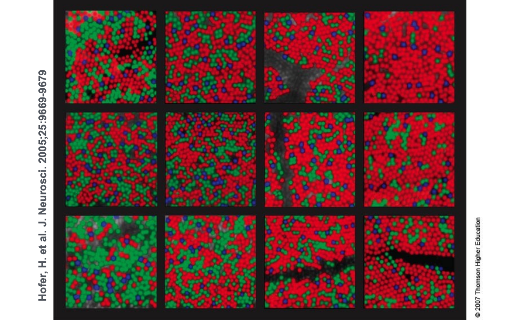
The proportions of the three cone types vary enormously from person to person: measuring the cone distribution at the edge of the fovea in 12 people with normal colour vision, the percentage of each cone type varies quite noticeably.
The tristimulus theory of colour
We now have three detectors (the S, M and L cones), each with a different spectral response curve.
A key fact about the human visual system:
The eye does not measure, and the brain does not receive, information about each individual wavelength.
The eye only “sees” three response values (S, M, L) — that is the only information the brain has.
4 Metamerism
Metamerism is a core concept in colour science: two different spectral distributions that look like the same colour to the human eye.
Metamers
Metamers are two different spectra (∞-dimensional) that project onto the same (S, M, L) response (3-dimensional).
They have the same colour as far as the human eye is concerned.
$$ \underbrace{s_1(\lambda) \neq s_2(\lambda)}_{\infty\text{-dimensional spectrum}} \quad \Longrightarrow \quad \underbrace{(S_1, M_1, L_1) = (S_2, M_2, L_2)}_{3\text{-dimensional response}} $$The existence of metamers is crucial for colour reproduction:
- You do not have to reproduce the complete spectrum of a real-world scene
- For example, a metamer can reproduce the perceived colour of a real scene on a display with only three colour pixels
Metamerism is exactly the theory behind colour matching. A photograph of the sun displayed in some way on a monitor looks practically the same colour, yet their spectra are completely different.
5 Color Reproduction / Matching
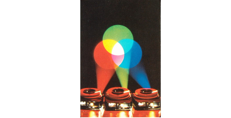
Additive colour
Given a set of primary lights, each with its own spectral distribution (for example the R, G and B pixels of a display): $s_R(\lambda), s_G(\lambda), s_B(\lambda)$.
Adjust the brightness of these lights and add them together:
$$ R \, s_R(\lambda) + G \, s_G(\lambda) + B \, s_B(\lambda) $$Colour can then be described by three scalar values: $R, G, B$.
The additive matching experiment
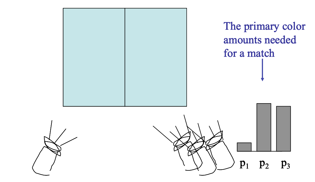
The apparatus: on the left is the test light to be matched, on the right are three primary lights $p_1, p_2, p_3$. The observer adjusts the intensities of the three primaries until the two sides look exactly the same.
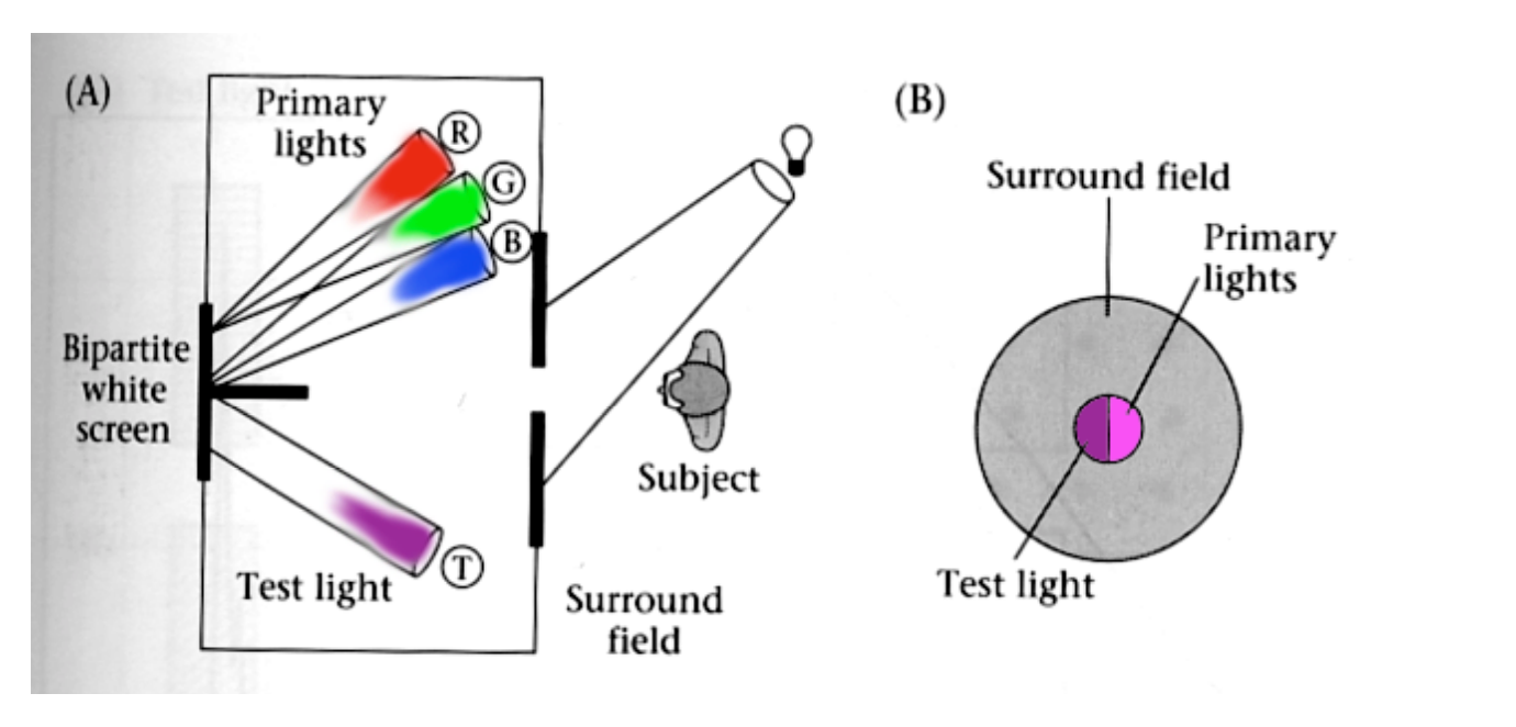
What gets recorded is “the amount of each primary needed to match” — this set of numbers defines the colour of that test light.
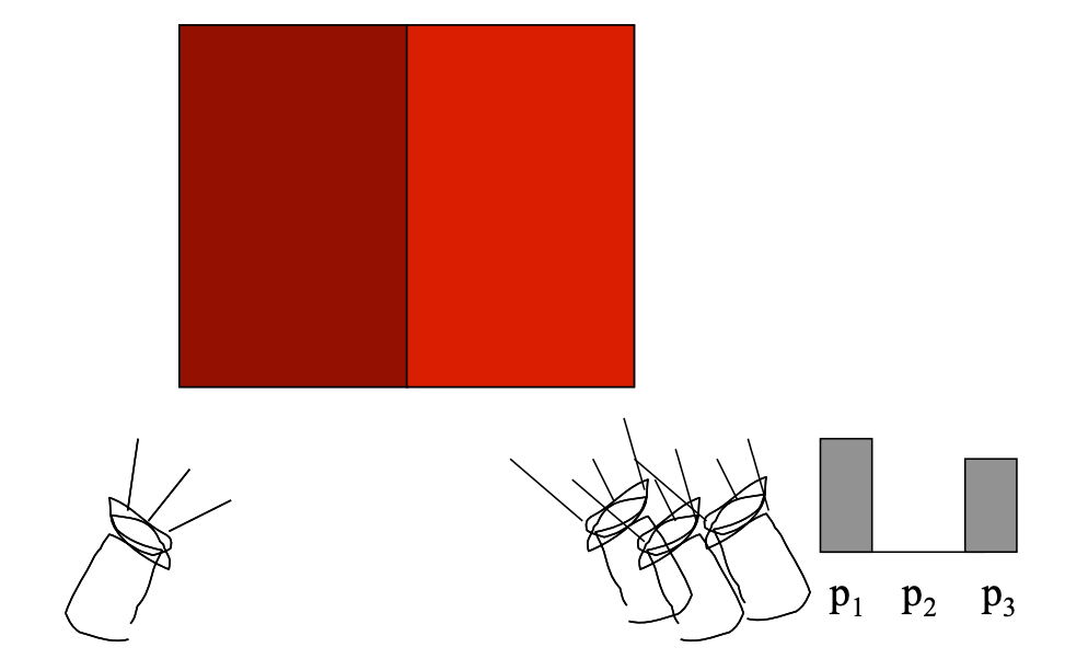
Experiment 2: the negative-value problem
Some test lights cannot be produced by “adding” the three primaries. In that case the observer adds one of the primaries to the test-light side and keeps adjusting.
We say a “negative” amount of $p_2$ is needed to match, because it was added to the test-light side.
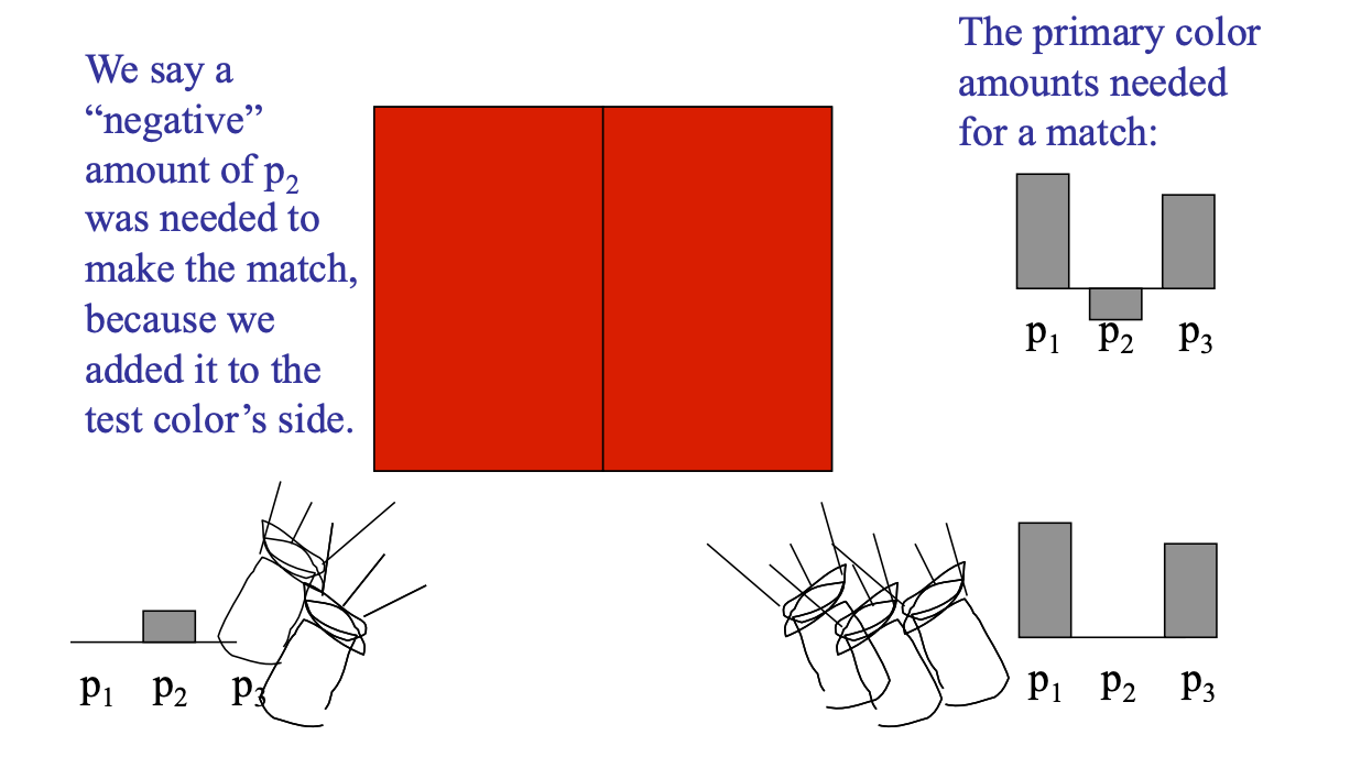
This negative-value phenomenon matters: it shows that no set of real three primaries can cover all the colours the human eye can see. This is precisely the motivation for introducing “imaginary primaries” in CIE XYZ.
The CIE RGB colour matching experiment
The apparatus is the same as the additive matching experiment above, except that:
- The primaries are monochromatic light (a single wavelength)
- The test light is monochromatic too
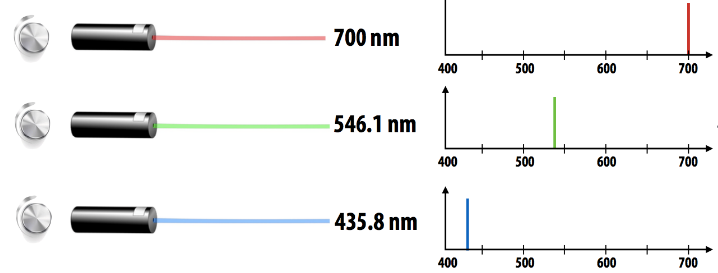
CIE RGB colour matching functions
The plot below shows: to match monochromatic light of a given wavelength on the x-axis, how much of each CIE RGB primary must be combined.
They are written $\bar{r}(\lambda), \bar{g}(\lambda), \bar{b}(\lambda)$.
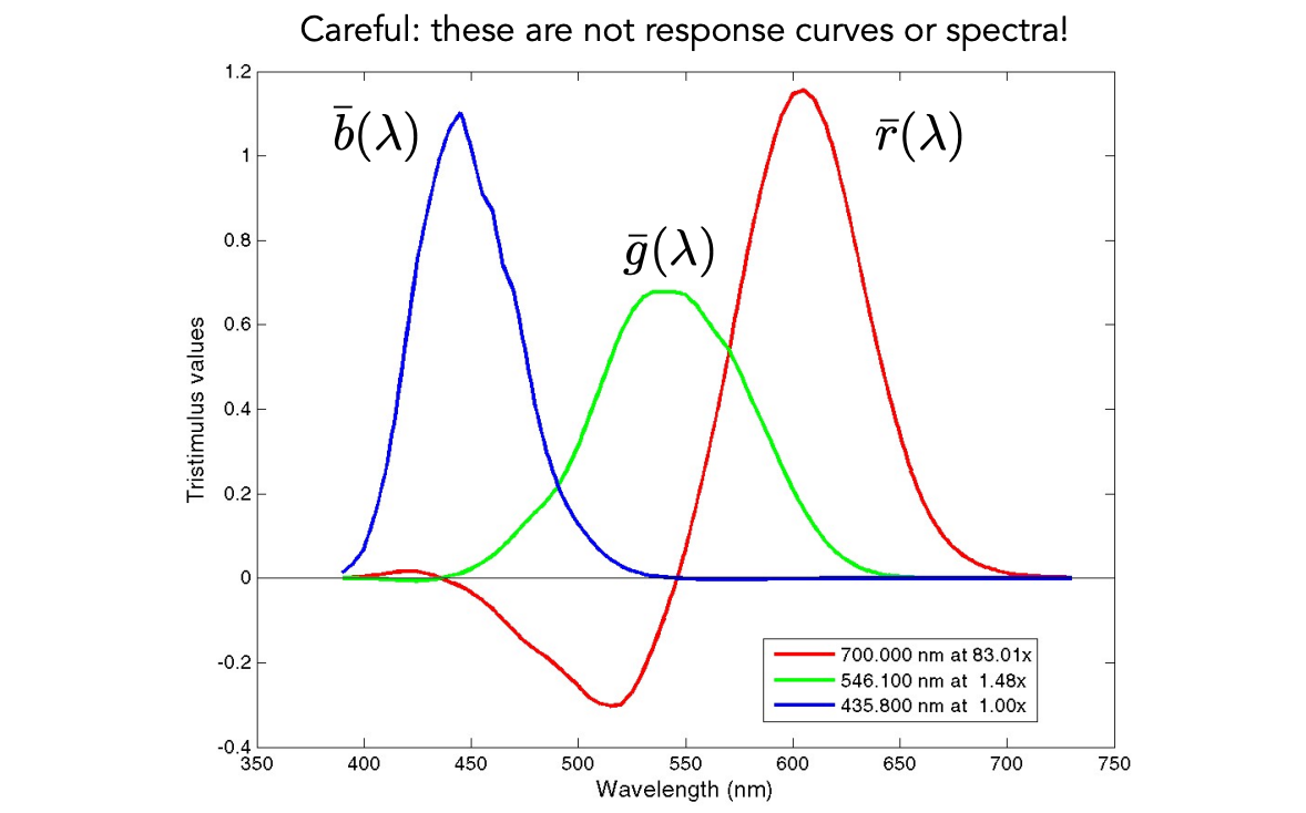
Careful: these are not response curves, and not spectra! They are “the amounts needed to match” — do not confuse them with the sensitivity curves of the cones.
Reproducing colour with matching functions
For any spectrum $s(\lambda)$, its perceived colour is matched by scaling the CIE RGB primaries with the following formulas:
$$ R_{\text{CIE RGB}} = \int s(\lambda) \, \bar{r}(\lambda) \, d\lambda $$$$ G_{\text{CIE RGB}} = \int s(\lambda) \, \bar{g}(\lambda) \, d\lambda $$$$ B_{\text{CIE RGB}} = \int s(\lambda) \, \bar{b}(\lambda) \, d\lambda $$Essentially it is a “spectrum × matching function” integral — projecting an infinite-dimensional spectrum down onto three colour values.
Once again: these are not response curves, and not the spectra of the primaries!
6 Color Spaces
A standard colour space: sRGB
- It makes one particular display’s RGB the standard
- Other colour devices emulate that display through calibration
- Widely adopted today
- The gamut is limited
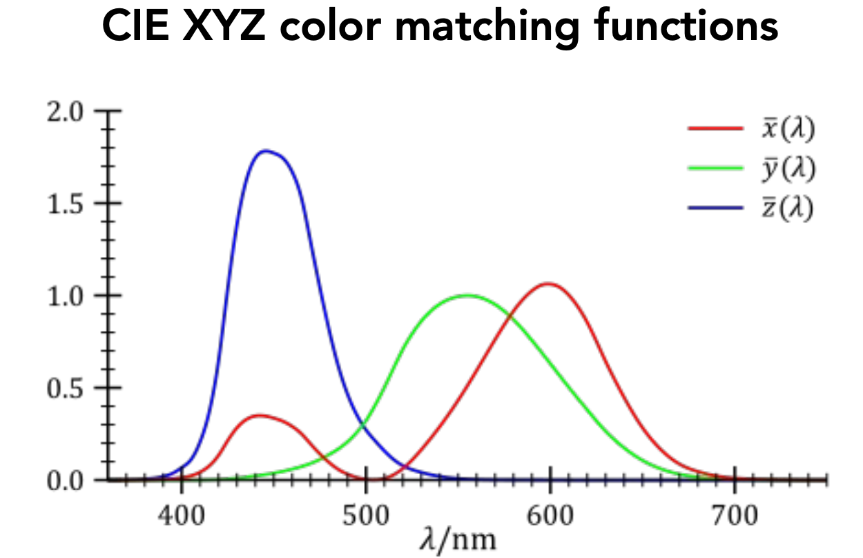
A universal colour space: CIE XYZ
A set of imaginary standard primaries $X, Y, Z$:
- Primaries with these matching functions do not exist (they are a mathematical construction, not real light)
- $Y$ is luminance — the lightness/darkness independent of colour
The design goals are:
- Matching functions strictly positive (avoiding the negative-value problem of CIE RGB)
- Spanning all observable colours
Separating luminance from chromaticity
| Quantity | Definition |
|---|---|
| Luminance | $Y$ |
| Chromaticity | $x, y, z$, defined as |
Since $x + y + z = 1$, only two of the three need to be stored.
Usually $x$ and $y$ are chosen, giving $(x, y)$ coordinates at a particular luminance $Y$.
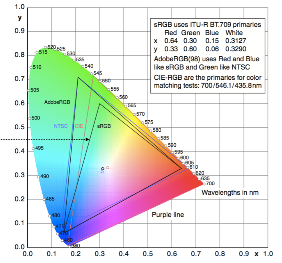
The CIE chromaticity diagram
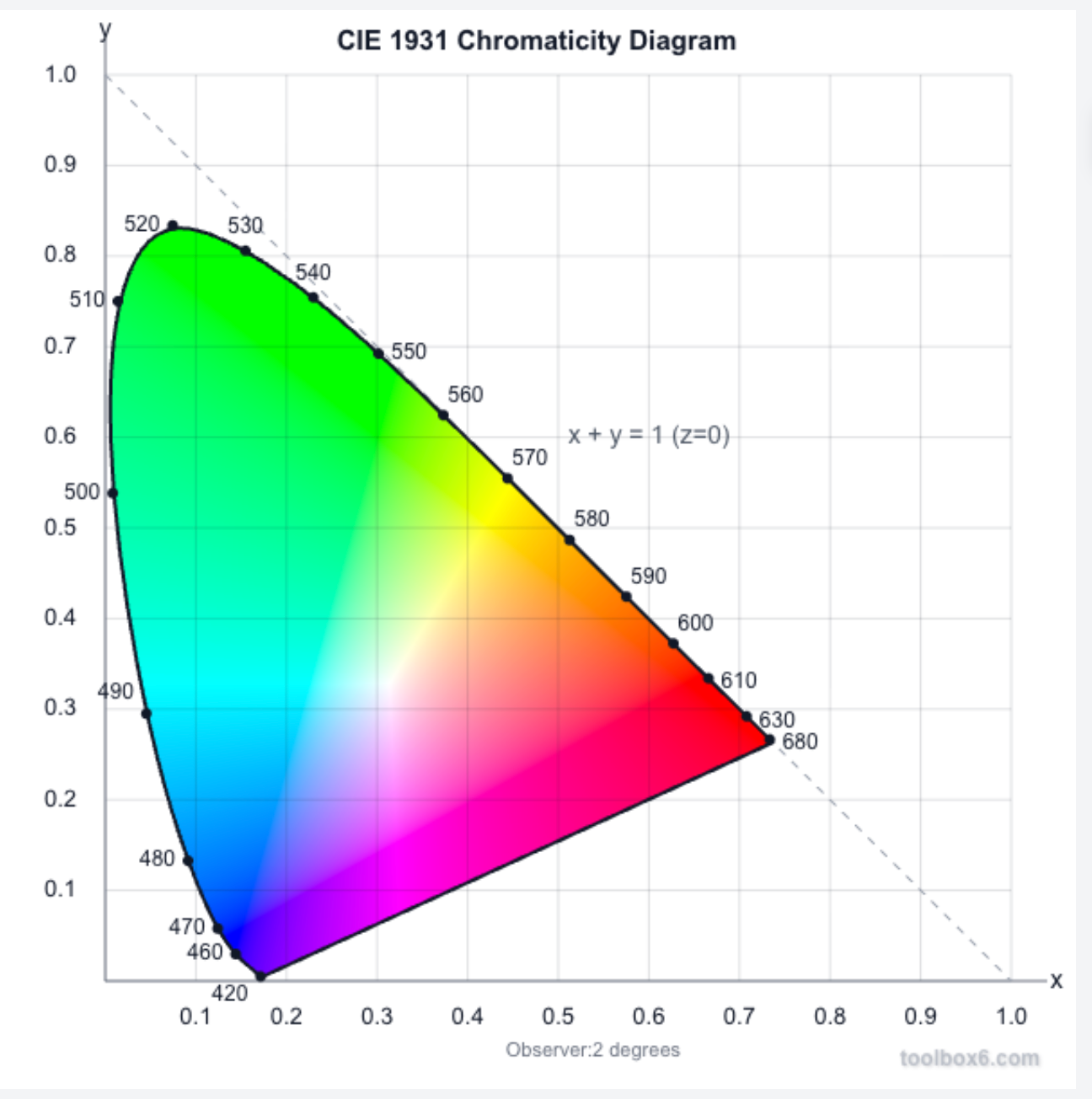
| Region | Meaning |
|---|---|
| Curved boundary | Called the spectral locus, corresponding to monochromatic light — each point is a pure colour of a single wavelength |
| Interior | Every colour is less than pure, i.e. a mixture |
| Centroid $(1/3, 1/3)$ | White |
Gamut
A gamut is the set of chromaticities a set of primaries can generate.
Different colour spaces represent different colour ranges, so they have different gamuts — they cover different regions of the chromaticity diagram.
sRGB is the colour space commonly used on the internet, but its gamut is only a small triangle in the chromaticity diagram.
Perceptually organized colour spaces
The spaces in the previous sections are defined by physics / matching (RGB, XYZ). Artists and colour pickers care about a different set of axes — ones that map directly onto how humans perceive colour.
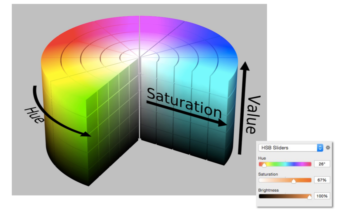
HSV colour space (Hue-Saturation-Value)
Its axes correspond to the artistic characteristics of colour, and it is widely used in “colour pickers”.
The perceptual dimensions of colour
| Dimension | Meaning | Colorimetric counterpart | Artist’s counterpart |
|---|---|---|---|
| Hue | The “kind” of colour, independent of attributes | Dominant wavelength | The chosen pigment colour |
| Saturation | “Colorfulness” | Purity | The proportion of pigment from the coloured tube |
| Lightness / Value | The overall amount of light | Luminance | A tint is brighter, a shade is darker |
CIELAB space (L*a*b*)
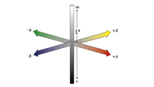
A commonly used colour space that strives for perceptual uniformity:
| Component | Meaning |
|---|---|
| $L^*$ | Lightness / brightness |
| $a^*$ | Opponent pair: red — green |
| $b^*$ | Opponent pair: blue — yellow |
Colours on opposite sides of the $a$ and $b$ axes are taken to be complementary.
Opponent colour theory
The dimensions of CIE LAB have a solid neurological basis:
The brain seems to encode colour along three axes early on: white — black, red — green, yellow — blue.
The white — black axis is lightness; the other two determine hue and saturation.
Evidence one (linguistic / intuitive):
You can have light green, dark green, yellow-green, blue-green, but you cannot have reddish green (it makes no sense) — so red is the opposite of green.
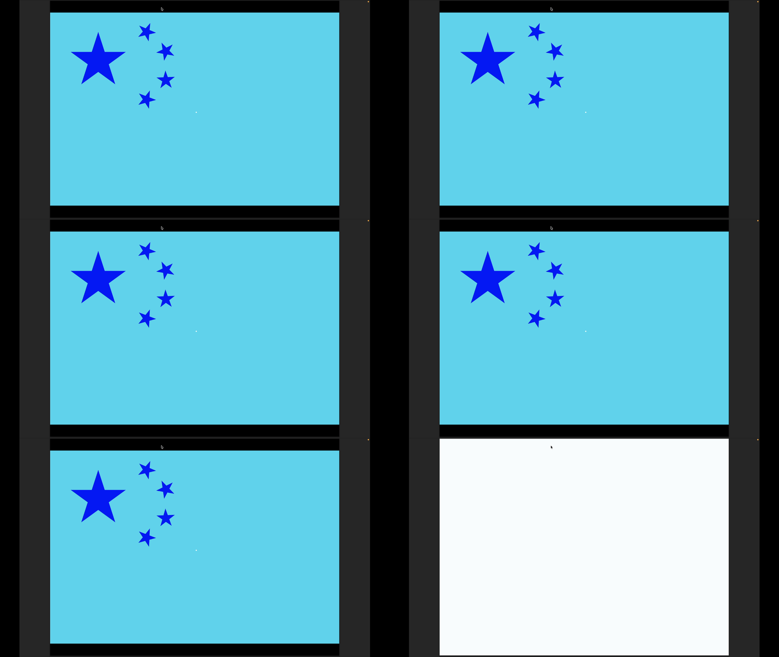
Evidence two (physiological): afterimages — stare at a colour for a while and then look at a white wall, and you will see its opposite colour.
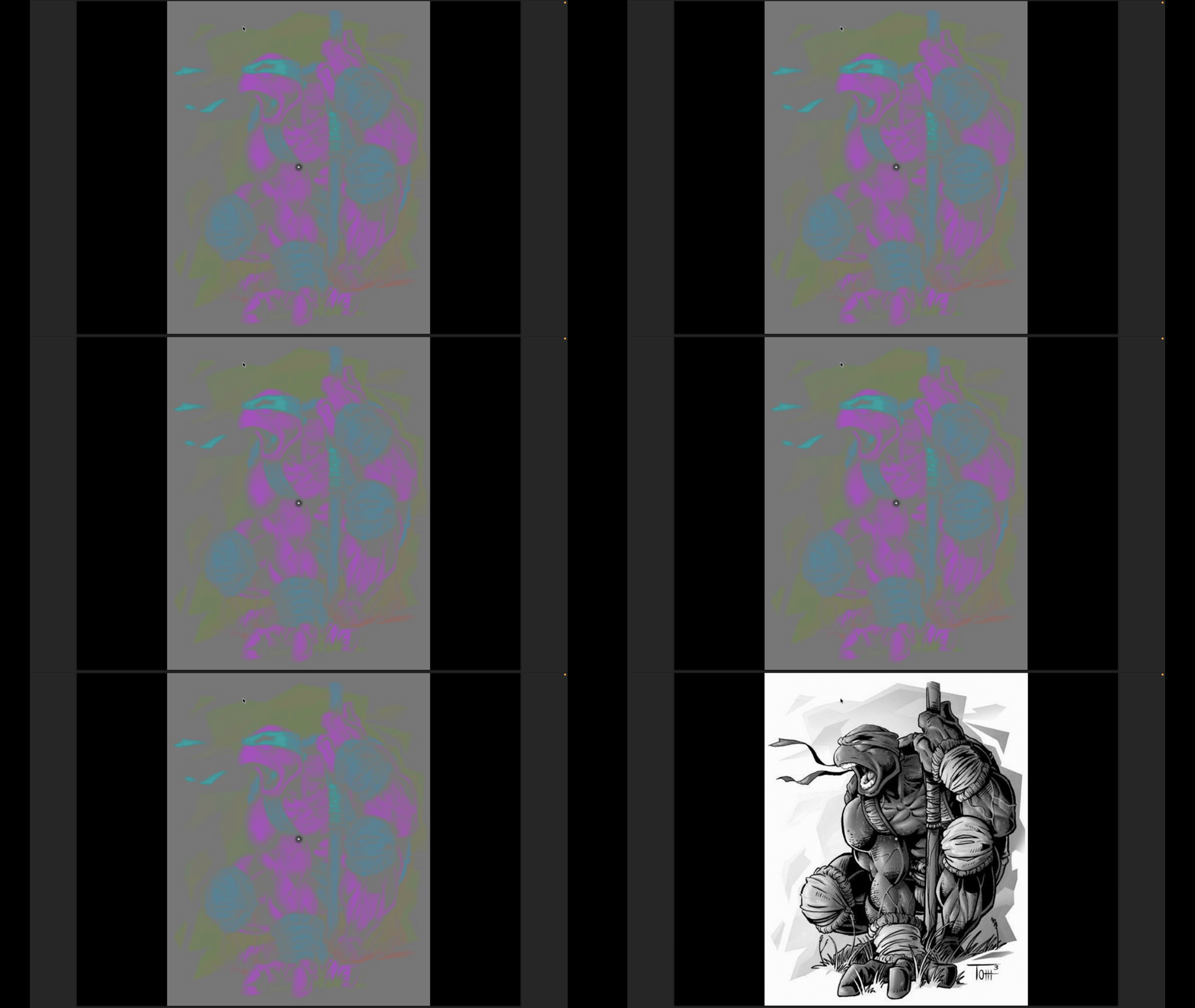
Adaptation and “everything is relative”
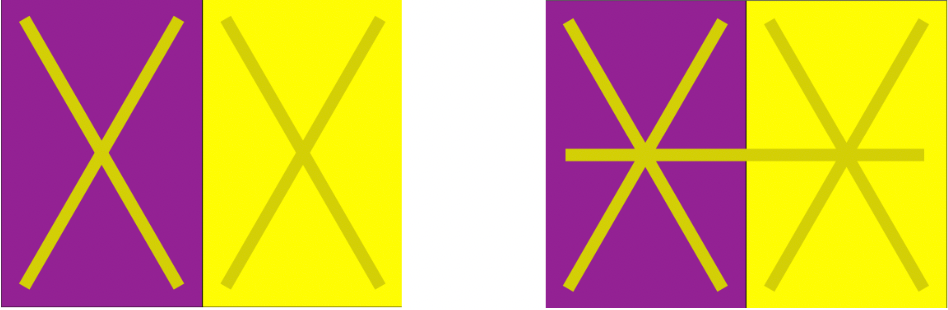
Human colour perception adapts: after being in a certain illumination for a long time, the visual system recalibrates “what white is”.
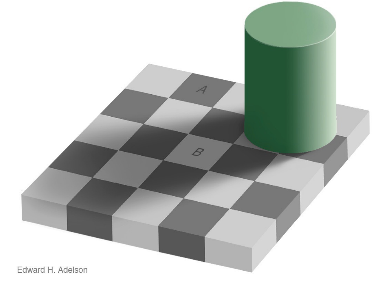
“Everything is relative” — the same colour patch is perceived as a completely different colour against a different background.
This explains why a render cannot just chase “numerically correct”: perception is the endpoint. It is also the fundamental reason HDR, tone mapping and colour management exist.
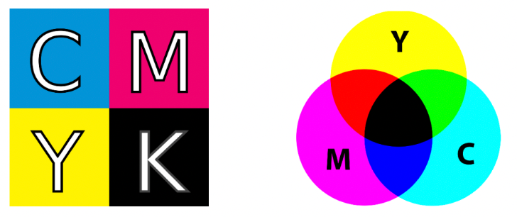
CMYK: a subtractive colour space
- Subtractive colour model: the more you mix, the darker it gets
- Cyan, Magenta, Yellow, Key (black)
- Widely used in printing
The question the lecture raises: if mixing C, M and Y can produce K, why do we still need K?
Summary
Lecture 20 lifts the viewpoint from “how do we compute geometry” up to “how much information is there” and “how does perception happen”:
| Topic | Key content |
|---|---|
| The plenoptic function | 7D: position $(\theta,\varphi,\lambda,t,V_x,V_y,V_z)$, covering rays at any position, direction, wavelength and instant — a complete description of “everything you can see” |
| Reducing to a light field | Drop time and colour to get 5D (3D position + 2D direction); in a vacuum ray intensity is constant along a line, so the position dimension degenerates, giving the 4D light field |
| Two-plane parameterization | $(s,t)$ position + $(u,v)$ direction; fixing $(s,t)$ and varying $(u,v)$ yields one image |
| Capturing light fields | Camera arrays (spatial multiplexing), integral imaging / microlens arrays (Lippmann, 1908) |
| Light field cameras | One pixel block = a set of directions; this buys computational refocusing and view synthesis at the cost of spatial resolution |
| SPD | The spectral power distribution describes energy by wavelength and adds linearly — the physical basis for computing lights separately and summing |
| Biological basis of colour | Rods (scotopic, greyscale only) and cones (photopic, three types S/M/L); the eye hands over only three response values |
| Metamerism | An ∞-dimensional spectrum projects onto the same 3D response; this is exactly why a three-primary display can reproduce the perceived colour of a real scene |
| Colour matching | Under additive colour, colour is described by three scalars $(R,G,B)$; the negative-value phenomenon shows no real three primaries can cover everything |
| CIE XYZ | Introduces imaginary primaries so the matching functions are strictly positive and span all visible colours; $Y$ is luminance |
| Chromaticity diagram and gamut | $x+y+z=1$ means only two need storing; the spectral locus is monochromatic light and the centroid is white; sRGB’s gamut is only a small triangle of it |
| Perceptual colour spaces | HSV maps onto artistic characteristics; CIELAB strives for perceptual uniformity, with $a^*$ and $b^*$ as opponent axes |
| Opponent colour theory | The white–black, red–green and yellow–blue axes, supported by both linguistic and afterimage evidence |
| Chromatic adaptation | The visual system recalibrates “what white is”, so the same patch is perceived differently against different backgrounds — perception is the endpoint of rendering |
This post is note #11 in the GAMES101 - Modern Computer Graphics learning series.