Instructor: Lingqi Yan | UCSB Bilibili: https://www.bilibili.com/video/BV1X7411F744 Lectures covered: Lecture 10 (Geometry 1: Introduction), Lecture 11 (Geometry 2: Curves and Surfaces), Lecture 12 (Geometry 3)
Geometry is an extremely important yet difficult topic in computer graphics. This post covers various ways to represent geometry (implicit and explicit), curves and surfaces (Bezier curves, B-splines, Bezier surfaces), mesh processing (subdivision, simplification, regularization) as well as the shadow mapping technique.

1 Geometry Representation Methods
In graphics, geometry representations fall into two broad categories: implicit and explicit. Each has its own pros and cons — there is no “best” representation; the choice depends on the task.
Implicit Geometry
Implicit representations are based on classifying points: a point satisfies some specified relationship (it does not tell you where the points are).
$$ f(x, y, z) = 0 $$For example, all points on a sphere satisfy:
$$ x^2 + y^2 + z^2 = 1 $$| Property | Description |
|---|---|
| Pros | Easy to test whether a point is inside or outside the surface (plug the point into the function and check the sign) |
| Cons | Hard to sample points on the surface directly (hard to know which points lie exactly on $f=0$) |
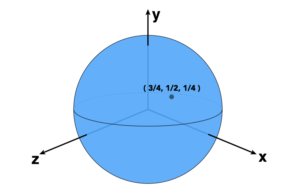
Inside/outside test example: for the sphere $f(x,y,z) = x^2 + y^2 + z^2 - 1$, test whether the point $(3/4, 1/2, 1/4)$ is inside:
$$ f(3/4, 1/2, 1/4) = (3/4)^2 + (1/2)^2 + (1/4)^2 - 1 = 9/16 + 1/4 + 1/16 - 1 = -1/8 < 0 $$The result is negative, meaning the point is inside the sphere.
Explicit Geometry
In explicit representations, all points are given directly, or via a parameter mapping.
$$ f: \mathbb{R}^2 \to \mathbb{R}^3; \quad (u, v) \mapsto (x, y, z) $$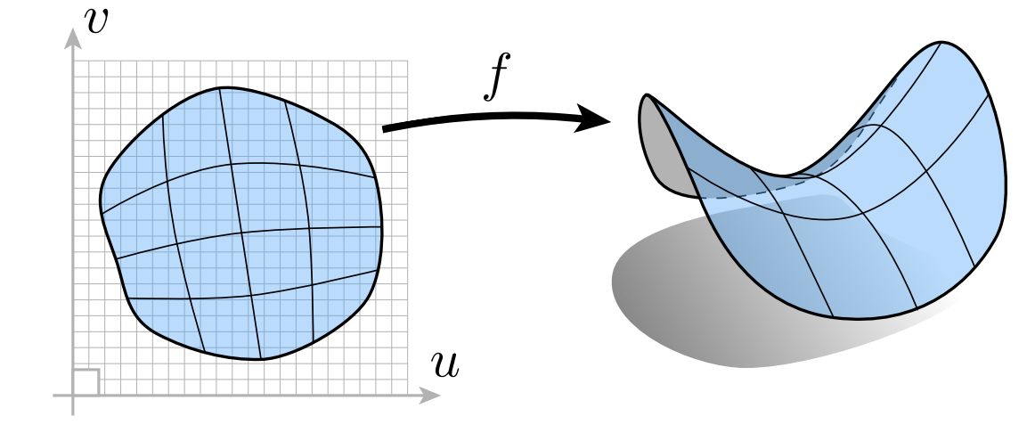
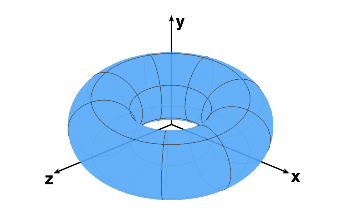
For example, a parametric representation of a torus:
$$ f(u, v) = \big((2 + \cos u)\cos v, \; (2 + \cos u)\sin v, \; \sin u\big) $$| Property | Description |
|---|---|
| Pros | Easy to sample (plug in $(u,v)$ values to get points on the surface) |
| Cons | Hard to test whether a point is inside or outside the surface |
Implicit vs Explicit Comparison
| Dimension | Implicit | Explicit |
|---|---|---|
| Representation | $f(x,y,z) = 0$ | $(x,y,z) = f(u,v)$ |
| Sampling | Hard | Easy |
| Inside/outside test | Easy (plug in and check the sign) | Hard |
| Typical use | Inside/outside tests, collision detection | Rendering, sampling surfaces |
“I hate meshes. I cannot believe how hard this is. Geometry is hard.” —— David Baraff (Pixar)
2 More Implicit Geometry Examples
There are many implicit representations in computer graphics:

Algebraic Surfaces
The surface is defined by the zero set of a polynomial in $x, y, z$.
| Shape | Equation |
|---|---|
| Sphere | $x^2 + y^2 + z^2 = 1$ |
| Torus | $\left(R - \sqrt{x^2 + y^2}\right)^2 + z^2 = r^2$ |
| Heart | $\left(x^2 + \frac{9y^2}{4} + z^2 - 1\right)^3 = x^2 z^3 + \frac{9y^2 z^3}{80}$ |
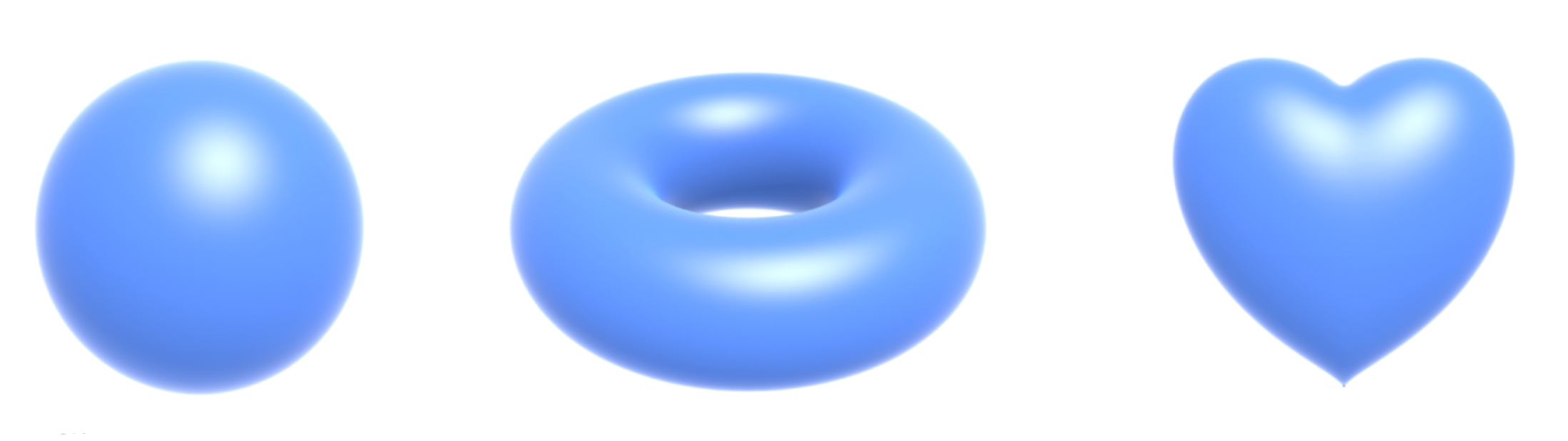
Limitation: complex shapes are hard to describe with a single algebraic equation (e.g. drawing a cow from the real world would be very difficult).
Constructive Solid Geometry (CSG)
Combine simple implicit primitives via Boolean operations to construct complex shapes.
| Operation | Symbol | Description |
|---|---|---|
| Union | $A \cup B$ | Union of two primitives |
| Intersection | $A \cap B$ | Intersection of two primitives |
| Difference | $A - B$ | Subtract B from A |
CSG Boolean expressions can be expressed with simple function operations:
- Union: $\min(f_A, f_B) = 0$
- Intersection: $\max(f_A, f_B) = 0$
- Difference: $\max(f_A, -f_B) = 0$
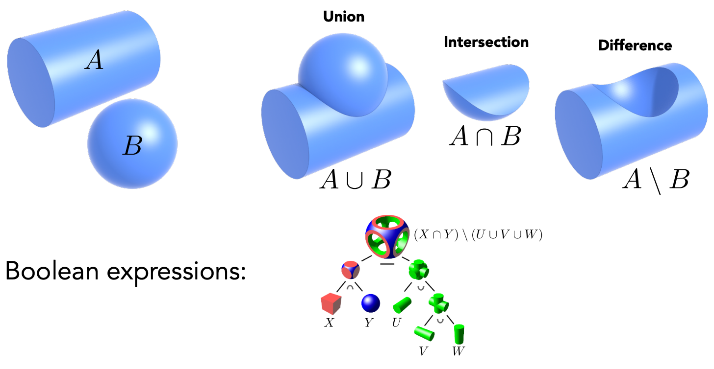
CSG is widely used in CAD modeling — very complex models can be built by combining simple primitives.
Distance Functions / SDF
A distance function gives the minimum distance from any position to the surface of an object (optionally signed — the Signed Distance Function).
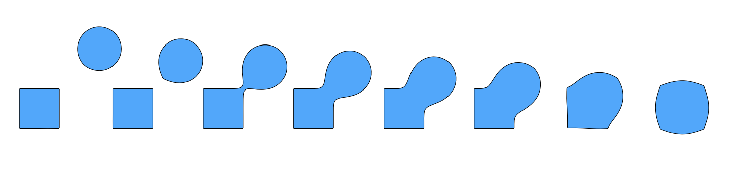
Core idea: instead of combining surfaces directly with Boolean operations, blend distance functions to fuse surfaces gradually.
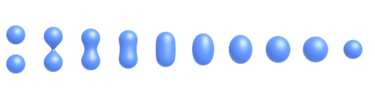
Blending distance functions: any two distance functions $d_1$, $d_2$ can be blended via linear interpolation:
$$ d_{blend} = (1 - t) \cdot d_1 + t \cdot d_2 $$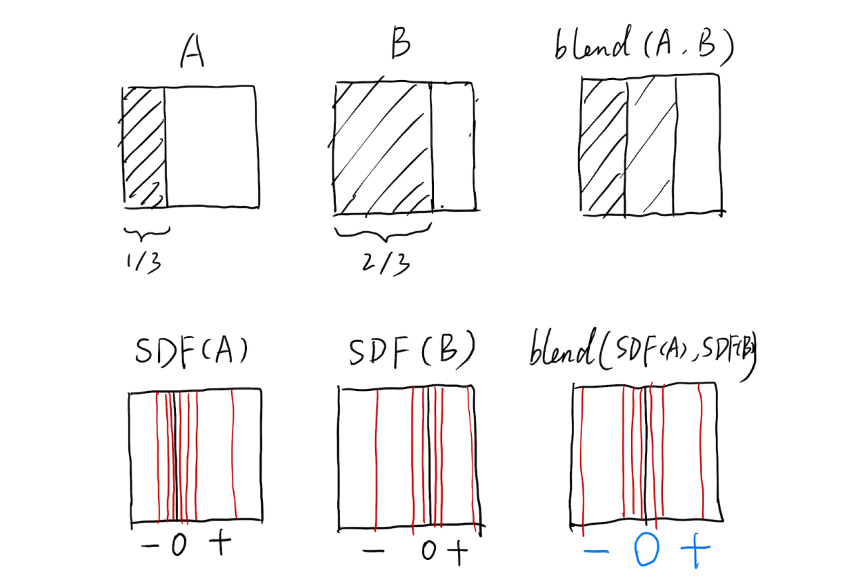
Advantages of SDF:
- Enables smooth fusion of shapes (e.g. droplet merging effects)
- Well suited for ray marching in ray tracing
- An entire scene can be built purely from distance functions
Level Sets
Level sets are a variant of distance functions where values are stored on a grid (like contour lines in 2D images).
- Store the function value $f(x, y, z)$ at each grid point
- The surface is the isosurface $f = 0$
- Smooth surfaces are obtained by interpolation
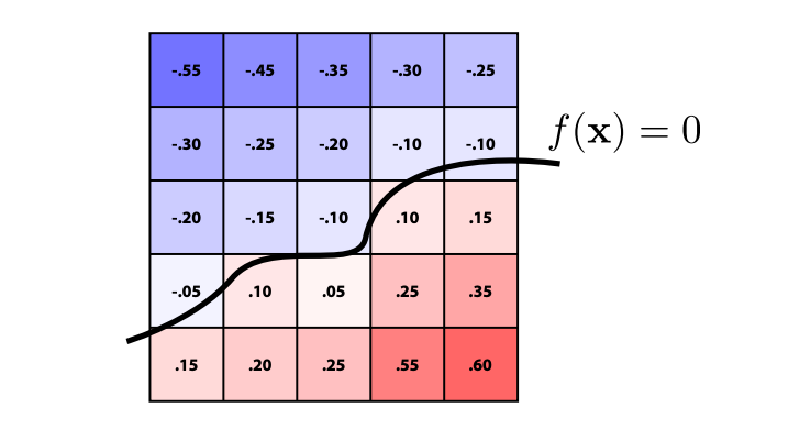
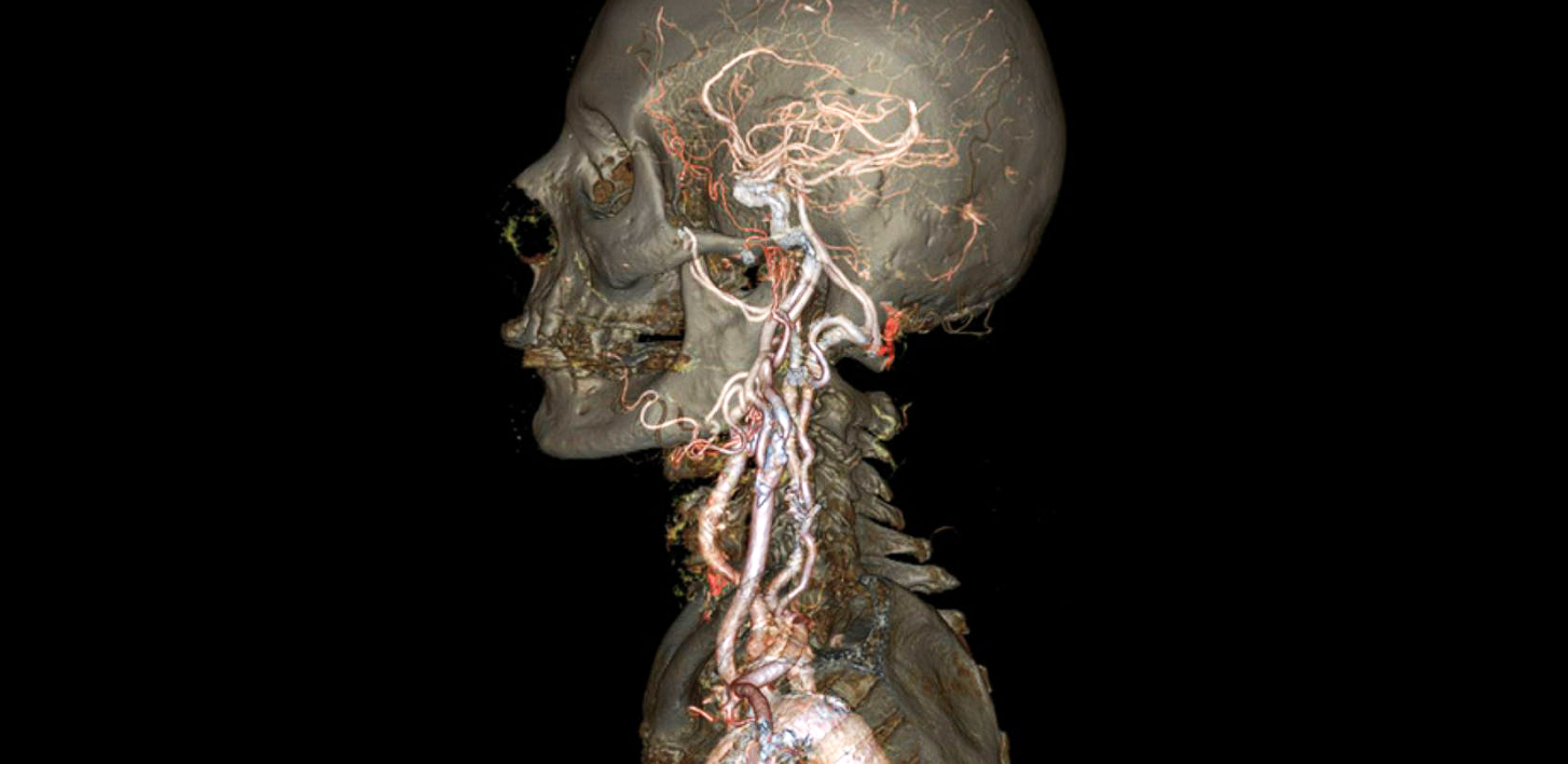
Applications: medical imaging (isosurface extraction from CT/MRI data), physical simulation (e.g. encoding the air-liquid interface distance in fluid simulation), etc.
Fractals
Fractal geometry exhibits self-similarity: parts resemble the whole in a statistical or exact sense.
Characteristics:
- Detail at all scales
- Hard to describe with conventional methods
- Suited to natural phenomena: snowflakes, mountains, coastlines, tree branches
Examples: Koch snowflake, Mandelbrot set, Sierpinski triangle, etc.
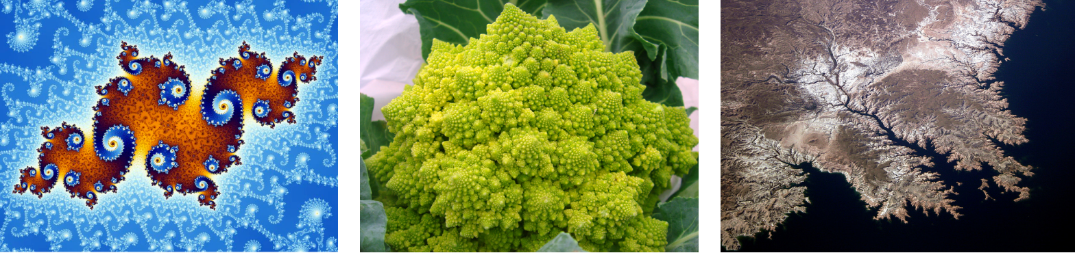
Problem: fractals show infinite detail when zoomed in, making sampling and rendering difficult.
Implicit Representation Summary
| Type | Content |
|---|---|
| Pros | Compact description (a single function); easy queries (inside test, distance to surface); good for ray-surface intersection; exact for simple shapes (no sampling error); handles topology changes (e.g. fluids) |
| Cons | Hard to model complex shapes |
3 More Explicit Geometry Examples
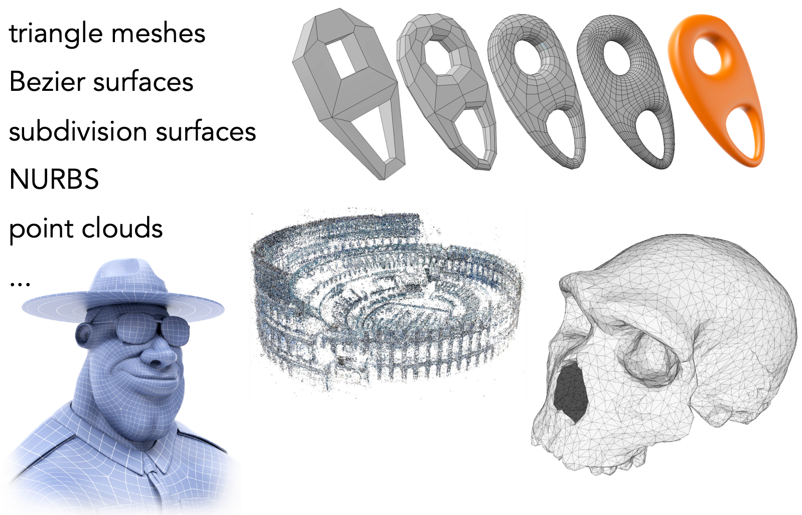
There are many explicit representations in graphics:
Point Cloud
The simplest representation: a list of points $(x, y, z)$.
| Property | Description |
|---|---|
| Pros | Easy to represent any type of geometry; suited to very large datasets (far more than one point per pixel) |
| Cons | Hard to draw in undersampled regions; usually converted to a polygon mesh |
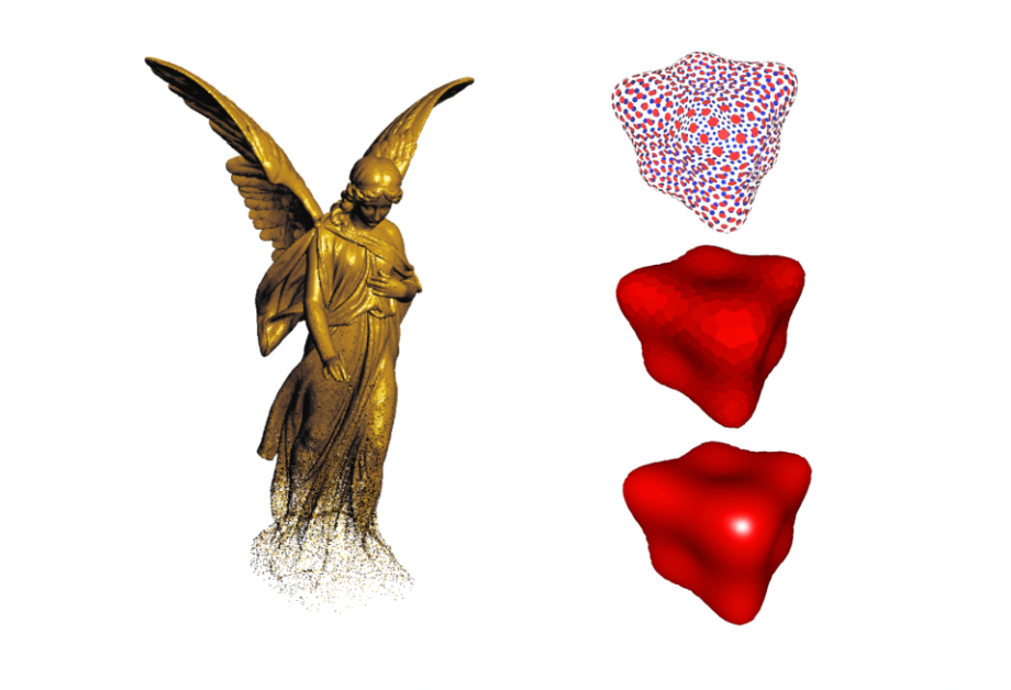
Point clouds are commonly used as the raw representation of 3D scans and LiDAR data.
Polygon Mesh
Stores vertices and polygons (usually triangles or quads).
| Property | Description |
|---|---|
| Pros | Easy to process/simulate; supports adaptive sampling; the most common representation in graphics |
| Cons | More complex data structure |
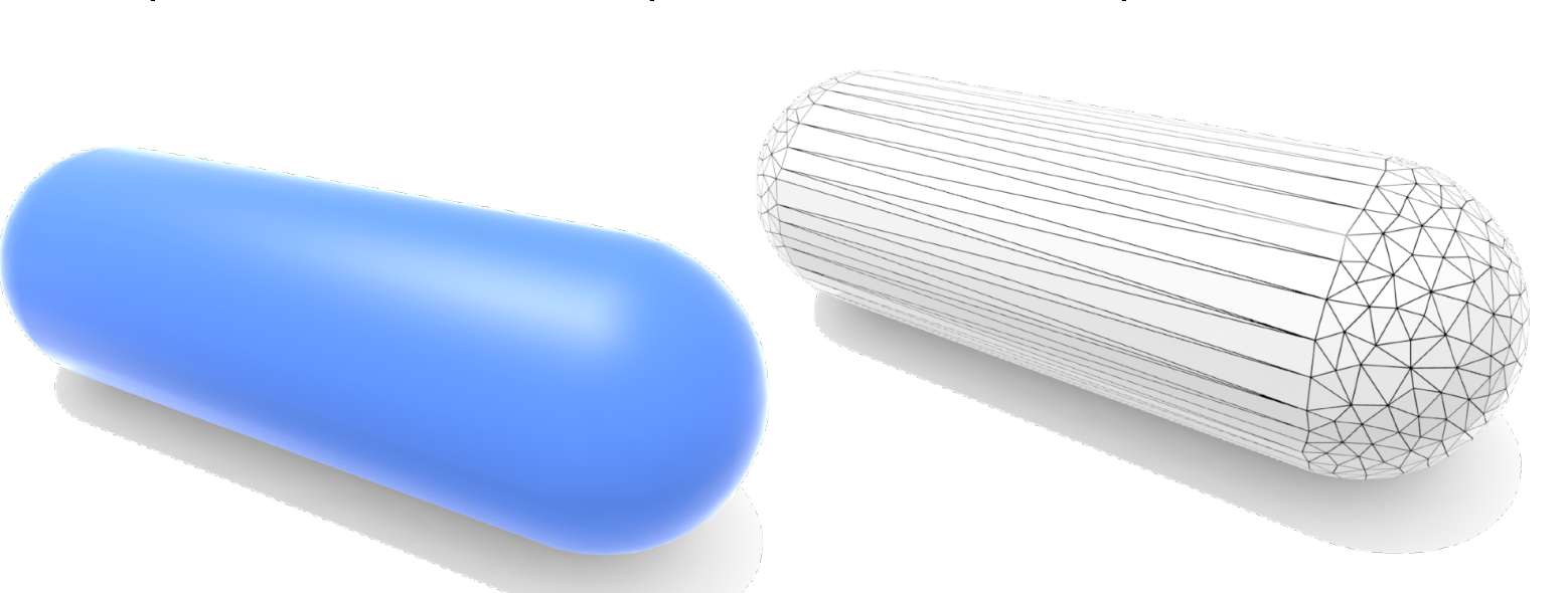
Wavefront .obj File Format
.obj is a common research file format — a text file specifying vertices, normals, texture coordinates and their connectivity.
# Vertices
v 1.000000 -1.000000 -1.000000
v 1.000000 -1.000000  1.000000
v -1.000000 -1.000000  1.000000
v -1.000000 -1.000000 -1.000000
...

# Texture coordinates
vt 0.748573 0.750412
...

# Normals
vn 0.000000 0.000000 -1.000000
...

# Faces (vertex index / texture index / normal index)
f 5/1/1 1/2/1 4/3/1
f 5/1/1 4/3/1 8/4/1
...
Key format:
v x y z: vertex positionvt u v: texture coordinatevn x y z: normal vectorf v/vt/vn v/vt/vn v/vt/vn: face (each vertex consists of vertex/texture/normal indices)
4 Bezier Curves
A Bezier curve is a parametric curve defined by control points, widely used in font design, path animation, vector graphics, etc.
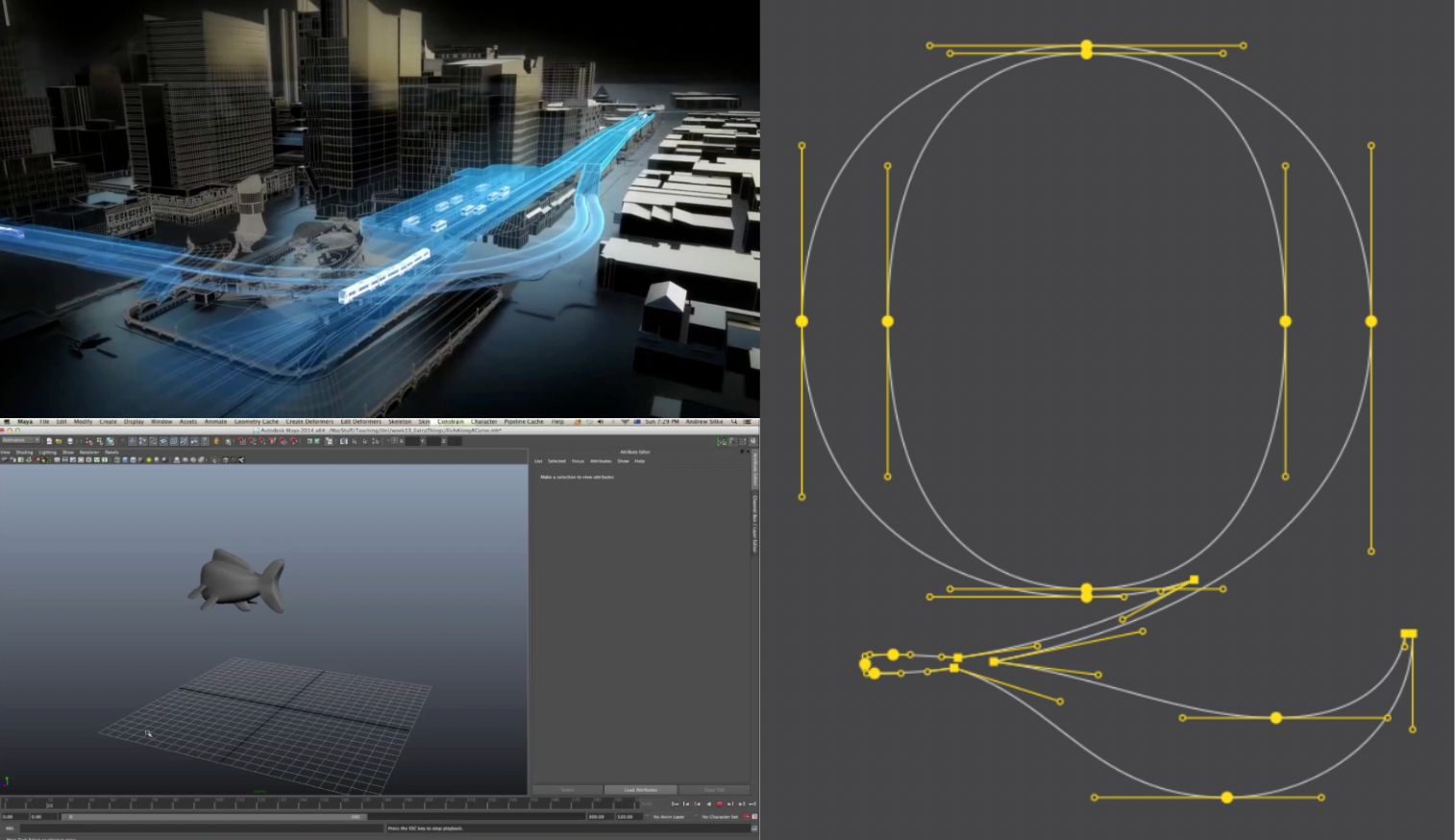
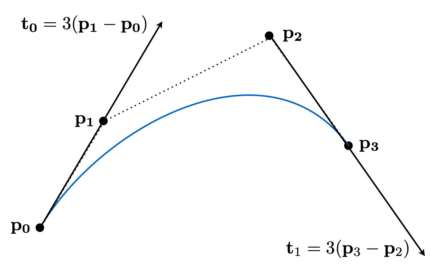
Defining a cubic Bezier curve with tangents: given control points $p_0, p_1, p_2, p_3$, the starting tangent is $t_0 = 3(p_1 - p_0)$ and the ending tangent is $t_1 = 3(p_3 - p_2)$.
The de Casteljau Algorithm
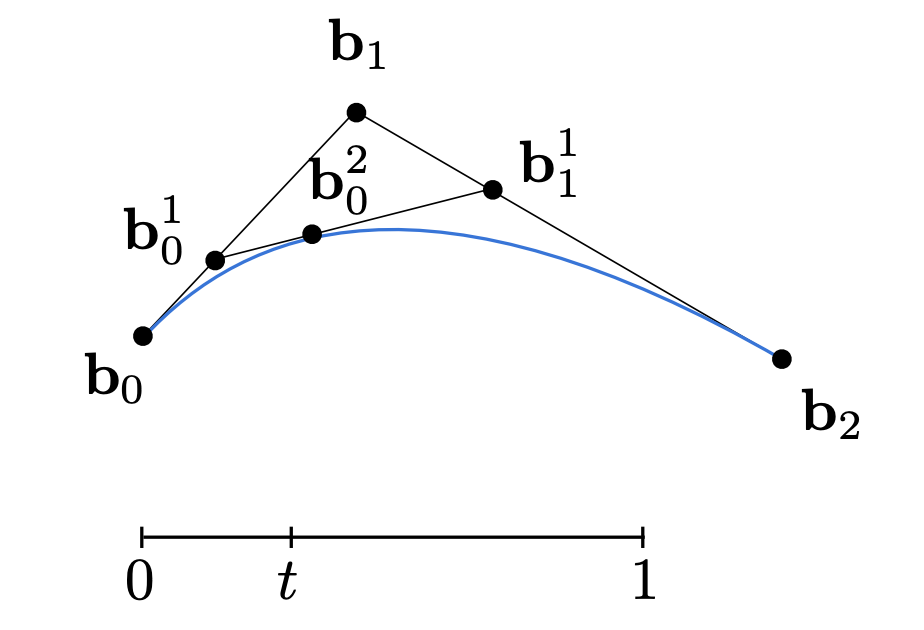
The de Casteljau algorithm computes points on a Bezier curve at parameter $t$ via recursive linear interpolation.
Quadratic Bezier curve example (3 control points $b_0, b_1, b_2$):
Step 1: take the point $b_0^1$ at ratio $t$ along $b_0 b_1$
$$ b_0^1(t) = (1 - t) b_0 + t b_1 $$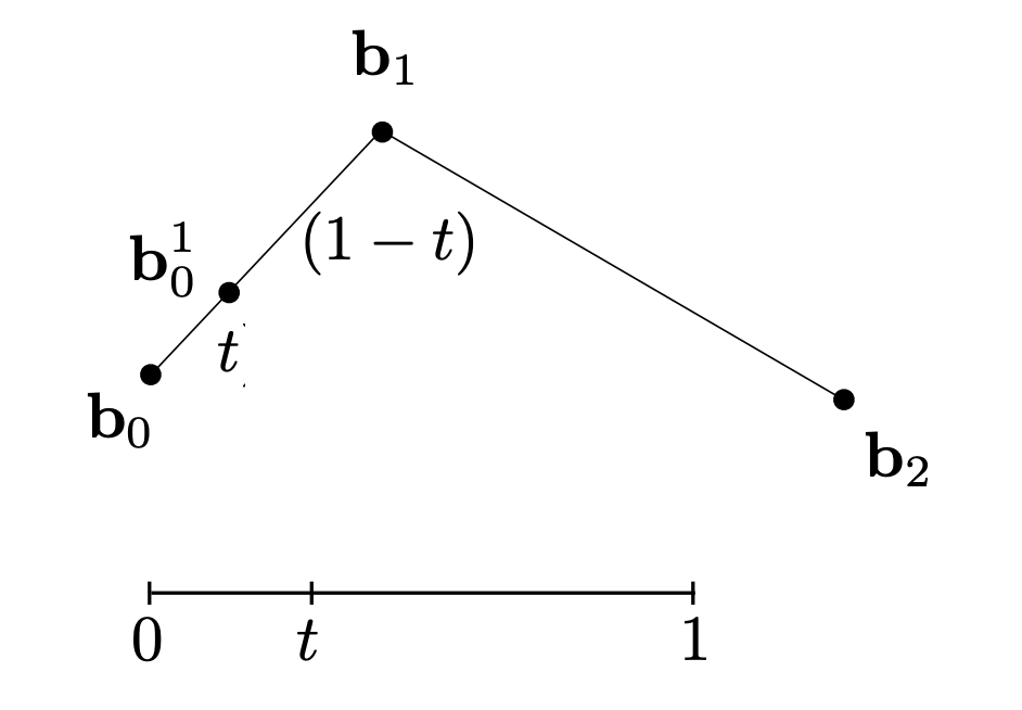
Step 2: take the point $b_1^1$ at ratio $t$ along $b_1 b_2$
$$ b_1^1(t) = (1 - t) b_1 + t b_2 $$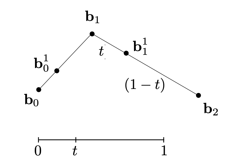
Step 3: take the point $b_0^2$ at ratio $t$ along $b_0^1 b_1^1$
$$ b_0^2(t) = (1 - t) b_0^1 + t b_1^1 $$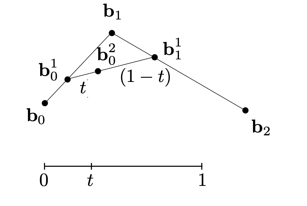
Step 4: repeat for every $t$ in $[0, 1]$ to obtain the whole curve.
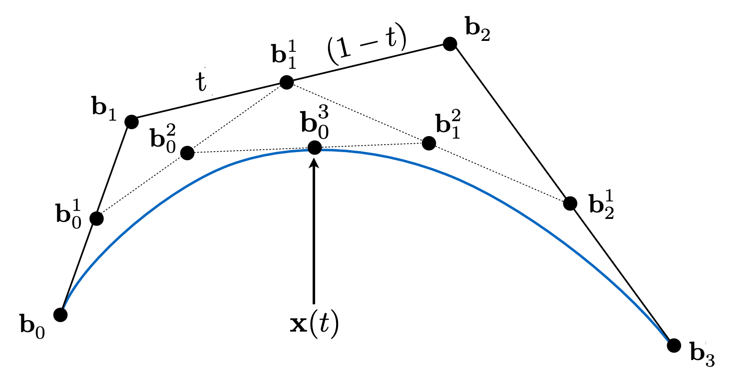
Cubic Bezier curve (4 control points $b_0, b_1, b_2, b_3$):
Apply the same recursive interpolation:
$$ \begin{aligned} b_0^1 &= (1-t) b_0 + t b_1 \\ b_1^1 &= (1-t) b_1 + t b_2 \\ b_2^1 &= (1-t) b_2 + t b_3 \\ b_0^2 &= (1-t) b_0^1 + t b_1^1 \\ b_1^2 &= (1-t) b_1^1 + t b_2^1 \\ b_0^3 &= (1-t) b_0^2 + t b_1^2 \end{aligned} $$$b_0^3(t)$ is the point on the curve at parameter $t$.
Algebraic Formula
de Casteljau yields a pyramid-like coefficient structure — each right-pointing arrow multiplies by $t$, each left-pointing arrow by $(1-t)$.
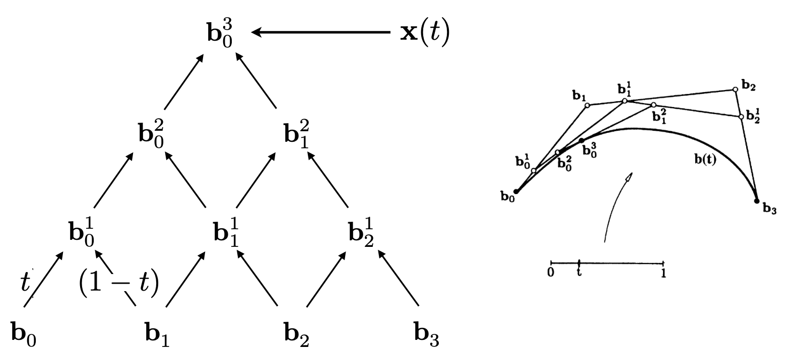
Expansion of a quadratic Bezier curve:
$$ \begin{aligned} b_0^1(t) &= (1-t) b_0 + t b_1 \\ b_1^1(t) &= (1-t) b_1 + t b_2 \\ b_0^2(t) &= (1-t) b_0^1 + t b_1^1 \\ &= (1-t)^2 b_0 + 2t(1-t) b_1 + t^2 b_2 \end{aligned} $$This mirrors $x^2+2xy+y^2 = (x+y)^2$; likewise the cubic case $(x+y)^3 = x^3 + 3x^2y + 3xy^2 + y^3$: the quadratic has 3 points, the cubic has 4.
Bernstein Polynomials and the General Formula
The Bernstein form of an $n$-degree Bezier curve:
$$ b^n(t) = \sum_{j=0}^{n} b_j \, B_j^n(t) $$where $B_j^n(t)$ is the Bernstein polynomial (basis function):
$$ B_i^n(t) = \binom{n}{i} t^i (1-t)^{n-i} $$$\binom{n}{i}$ is the binomial coefficient, $\binom{n}{i} = \frac{n!}{i!(n-i)!}$ — it assigns a “fair weight” to each control point.
Cubic Bezier curve ($n = 3$) expansion:
$$ b^n(t) = b_0 (1-t)^3 + b_1 \cdot 3t(1-t)^2 + b_2 \cdot 3t^2(1-t) + b_3 \cdot t^3 $$Cubic Bezier basis functions (Bernstein polynomials, $n=3$):
| Basis function | Expression |
|---|---|
| $B_0^3(t)$ | $(1-t)^3$ |
| $B_1^3(t)$ | $3t(1-t)^2$ |
| $B_2^3(t)$ | $3t^2(1-t)$ |
| $B_3^3(t)$ | $t^3$ |
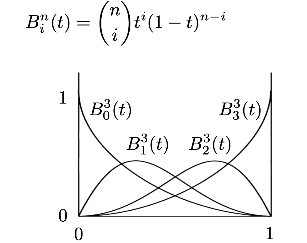
The Bernstein coefficients form Pascal’s triangle (binomial expansion coefficients):
        1          (n=0)
      1   1        (n=1)
    1   2   1      (n=2)
  1   3   3   1    (n=3)  ← cubic Bezier
1   4   6   4   1  (n=4)
These basis functions satisfy:
- Non-negativity: $B_i^n(t) \geq 0$ for $t \in [0, 1]$
- Partition of unity (sum to 1): $\sum_{i=0}^{n} B_i^n(t) = 1$ for any $t$
Properties of Bezier Curves
| Property | Description |
|---|---|
| Endpoint interpolation | The curve passes through the first and last control points. Cubic Bezier: $b(0) = b_0$, $b(1) = b_3$ |
| Tangent direction | The tangent at an endpoint is aligned with the control segment. Cubic Bezier: $b'(0) = 3(b_1 - b_0)$, $b'(1) = 3(b_3 - b_2)$ |
| Affine invariance | Transforming the curve affinely = transforming the control points then redrawing the curve |
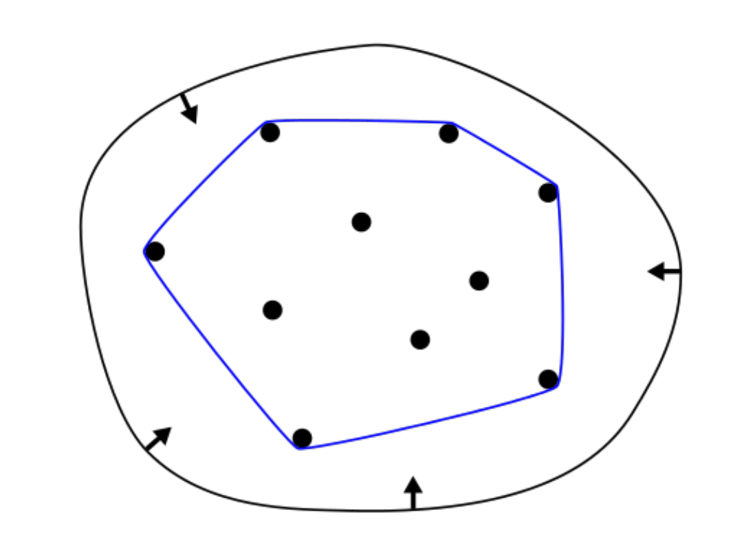
| Convex hull property | The curve always lies inside the convex hull of its control points |
Convex Hull: the smallest convex set containing a set of points. Imagine wrapping a rubber band around all points; the tightened rubber band is the convex hull.
Piecewise Bezier Curves
Problem: high-degree Bezier curves (many control points) are hard to control and rarely used in practice.
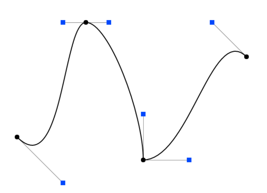
Solution: chain multiple low-degree Bezier curves together — the most common being piecewise cubic Bezier curves.
Piecewise cubic Bezier curves are widely used in font design, path definition, Illustrator, Keynote, etc. (like the pen tool).
Continuity of Piecewise Bezier Curves
Consider two Bezier curves:
- $a: [k, k+1] \to \mathbb{R}^N$ with control points $a_0, a_1, \ldots, a_n$
- $b: [k+1, k+2] \to \mathbb{R}^N$ with control points $b_0, b_1, \ldots, b_n$
| Continuity type | Condition | Description |
|---|---|---|
| $C^0$ continuous | $a_n = b_0$ | The two segments meet at the same position |
| $C^1$ continuous | $a_n = b_0 = \frac{1}{2}(a_{n-1} + b_1)$ | Same position and aligned tangents (continuous first derivative) |
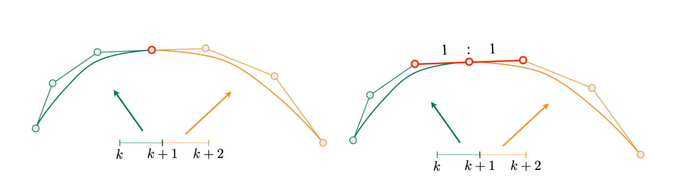
Geometric meaning of $C^1$: the junction $a_n(=b_0)$ is the midpoint of the second-to-last control point $a_{n-1}$ of the first segment and the second control point $b_1$ of the second segment.
5 B-splines
Spline definition: a continuous curve through a given set of points with a specified number of continuous derivatives. In short, a controlled curve.
B-splines stand for Basis Splines.
| Property | Description |
|---|---|
| Locality | Modifying one control point only affects the curve locally, not the whole curve (with Bezier, one control point affects the whole curve) |
| Satisfies all important Bezier properties | A superset of Bezier curves |
| Requires more information | Needs more parameters than Bezier curves |
B-spline vs Bezier curve:
| Dimension | Bezier | B-spline |
|---|---|---|
| Control point influence | Global (one control point affects the whole curve) | Local (one control point only affects nearby segments) |
| Flexibility | Lower | Higher |
| Complexity | Simpler | More complex |
| Relationship | A special case of B-splines | A generalization of Bezier curves |
Note: this course does not go deep into B-splines and NURBS, nor curve operations (e.g. degree elevation/reduction). For deeper content, see Prof. Hu Shimin’s course: https://www.bilibili.com/video/av66548502
6 Bezier Surfaces
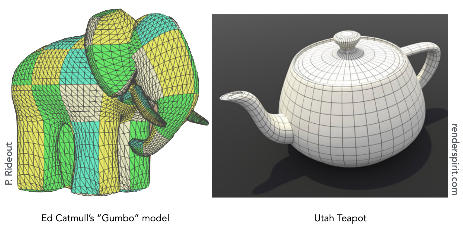
Extending Bezier curves to surfaces. Ed Catmull’s Gumbo model and the Utah Teapot are classic examples of Bezier surfaces.
Bicubic Bezier Surface Patch
A $4 \times 4$ array of control points defines one surface patch.
- Input: $4 \times 4 = 16$ control points
- Output: a 2D surface defined by parameters $(u, v) \in [0,1]^2$
Evaluating a Bezier Surface

Uses a separable 1D de Casteljau algorithm:
Goal: find the surface position at parameters $(u, v)$.
Step 1: evaluate the 4 Bezier curves in the $u$ direction separately with de Casteljau, obtaining one point per curve at $u$. This gives 4 “moving” control points.
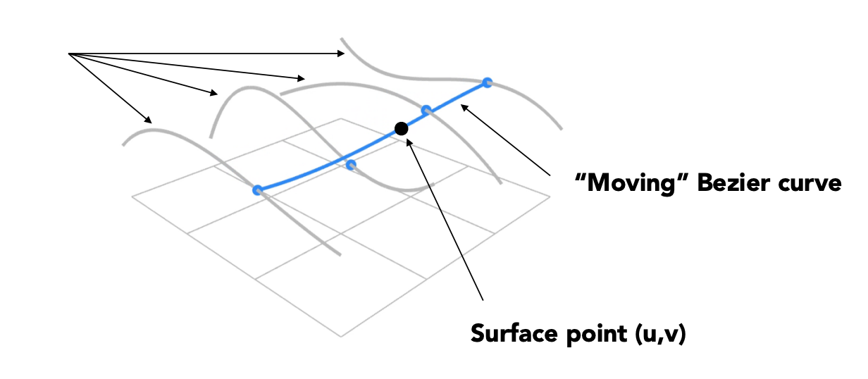
Step 2: form a new Bezier curve from these 4 control points and evaluate it in the $v$ direction with de Casteljau.
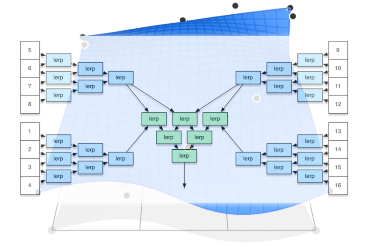
The resulting point is the surface position at $(u, v)$:
$$ \text{Surface}(u, v) = \sum_{i=0}^{3} \sum_{j=0}^{3} b_{ij} \, B_i^3(u) \, B_j^3(v) $$7 Mesh Subdivision
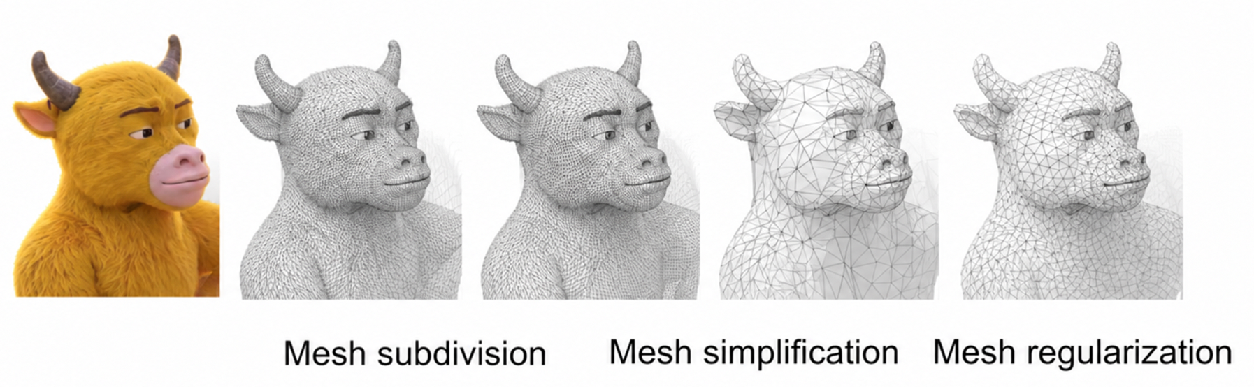
Mesh subdivision is an upsampling operation: it increases mesh resolution to make the surface smoother.
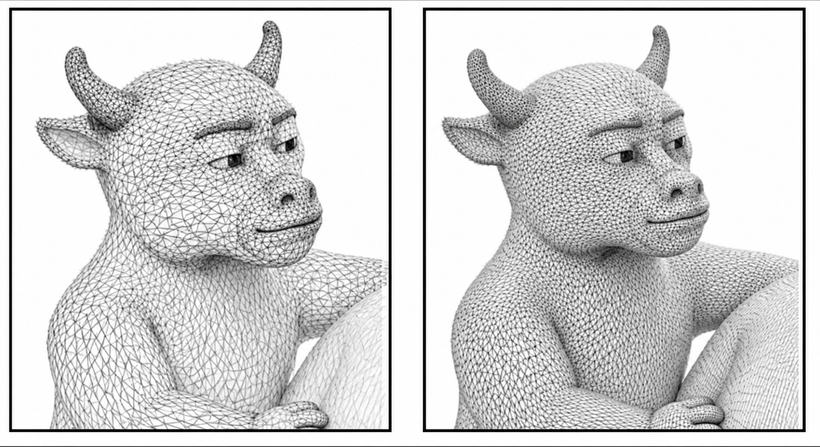
Loop Subdivision
Loop subdivision is the common subdivision method for triangle meshes.
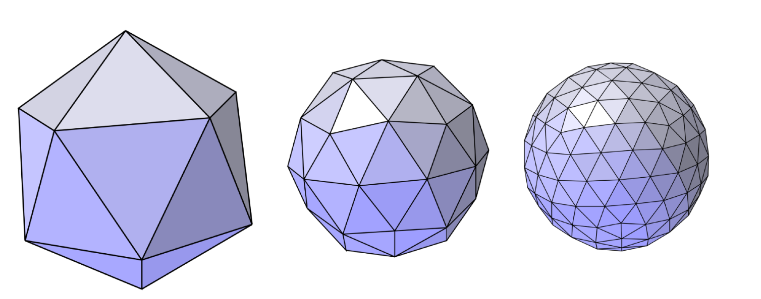
Core idea:
- Create more triangles (vertices)
- Adjust vertex positions to make the model smoother
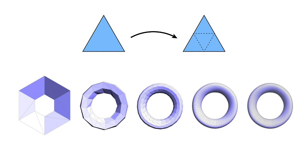
Step 1: split triangles
Split each triangle into 4 smaller triangles (connect the midpoints of the edges).
Step 2: update vertex positions
New and old vertices use different update rules.
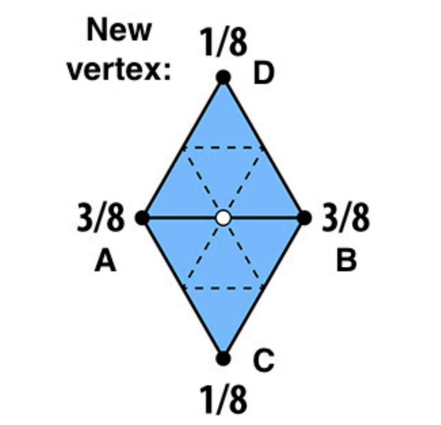
New vertex update (the new vertex lies on an edge):
$$ \text{New vertex position} = \frac{3}{8}(A + B) + \frac{1}{8}(C + D) $$where $A$, $B$ are the old vertices at the two ends of the edge, and $C$, $D$ are the opposite vertices of the two triangles adjacent to the edge.
Old vertex update (for a vertex of degree $n$):
$$ \text{New position} = (1 - n \cdot u) \cdot \text{old position} + u \cdot \sum \text{neighbor positions} $$where:
- $n$: the degree of the vertex (number of adjacent vertices / incident edges)
- $u$: weight; $u = 3/16$ when $n = 3$, and $u = \frac{3}{8n}$ when $n > 3$
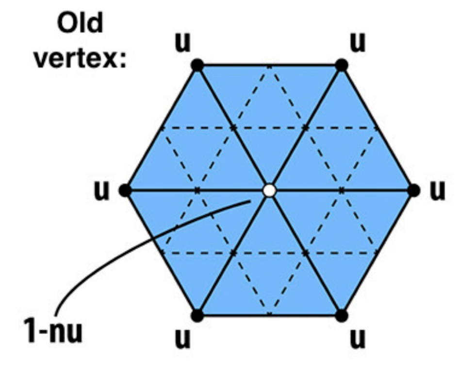
New vertices are placed by weighted averaging; old vertices are updated by a weighted combination of their own position and neighboring old vertices (more of one’s own information or more of the neighbors’ information). The full mesh is subdivided in the end.
Loop subdivision result:

Catmull-Clark Subdivision
Catmull-Clark subdivision works on general meshes (which may contain both triangles and quads).
Key concepts:
- Extraordinary vertex: a vertex whose degree (number of incident edges) is not 4
- The center of a triangle face is always an extraordinary vertex of degree 3
Step 1: subdivision operations
For each face:
- Add a face point to each face: the average of the face’s vertices
- Add an edge point to each edge: the average of the two endpoints and the two adjacent face points

Step 2: connect
Connect face points with edge points, subdividing each face into 4 quads.
Important properties:
- After one subdivision, all faces become quads
- The number of extraordinary vertices no longer increases after the first subdivision (each non-quad face introduces one extraordinary vertex, after which all faces are quads)
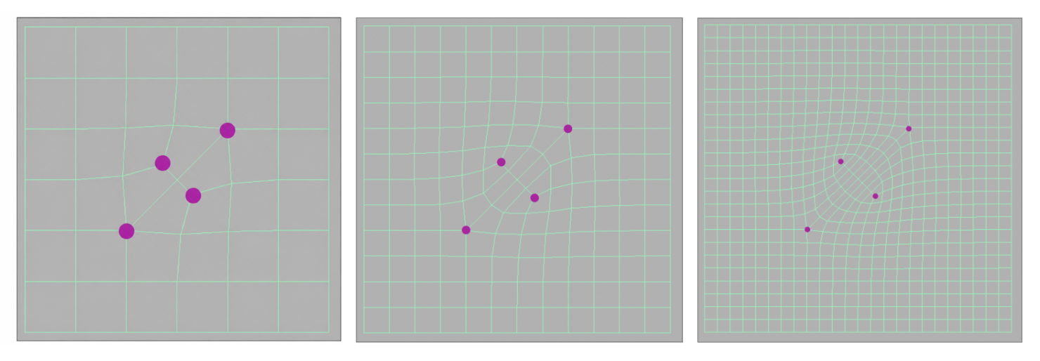
Thought question (the sample mesh in the slides): after one subdivision, 2 new extraordinary vertices are introduced (degree 3 and degree 5), and the number of non-quad faces becomes 0 — all non-quad faces disappear after one subdivision.
Catmull-Clark vertex update rules (quad meshes):
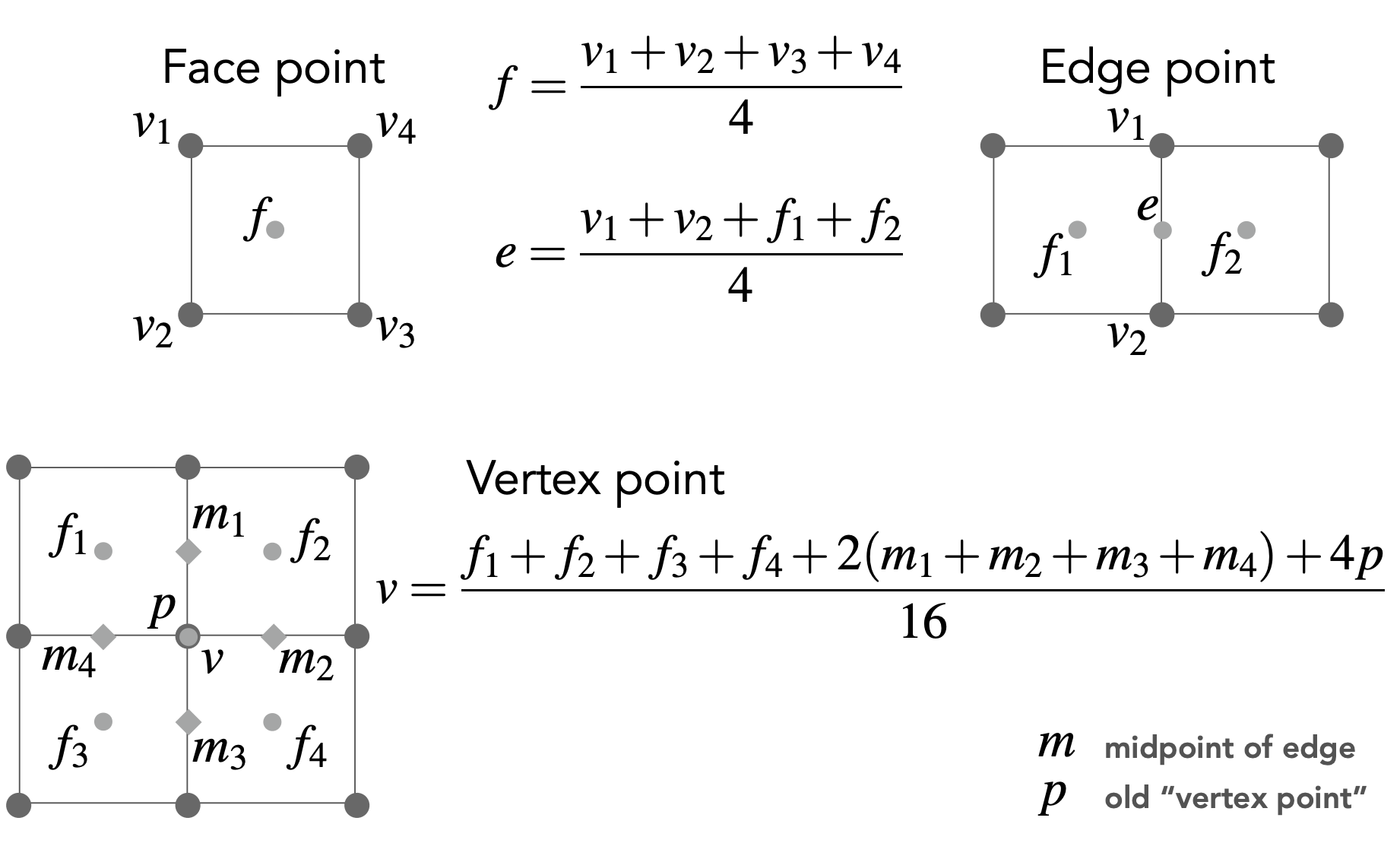
| Vertex type | Update formula |
|---|---|
| Face point | $f = \frac{v_1 + v_2 + v_3 + v_4}{4}$ |
| Edge point | $e = \frac{v_1 + v_2 + f_1 + f_2}{4}$ |
| Vertex point | $v = \frac{f_1 + f_2 + f_3 + f_4 + 2(m_1 + m_2 + m_3 + m_4) + 4p}{16}$ |
where:
- $f_1, f_2, f_3, f_4$: adjacent face points
- $m_1, m_2, m_3, m_4$: midpoints of adjacent edges
- $p$: the original vertex position
Convergence: after repeated subdivision, the overall shape and creases converge to a stable limit.
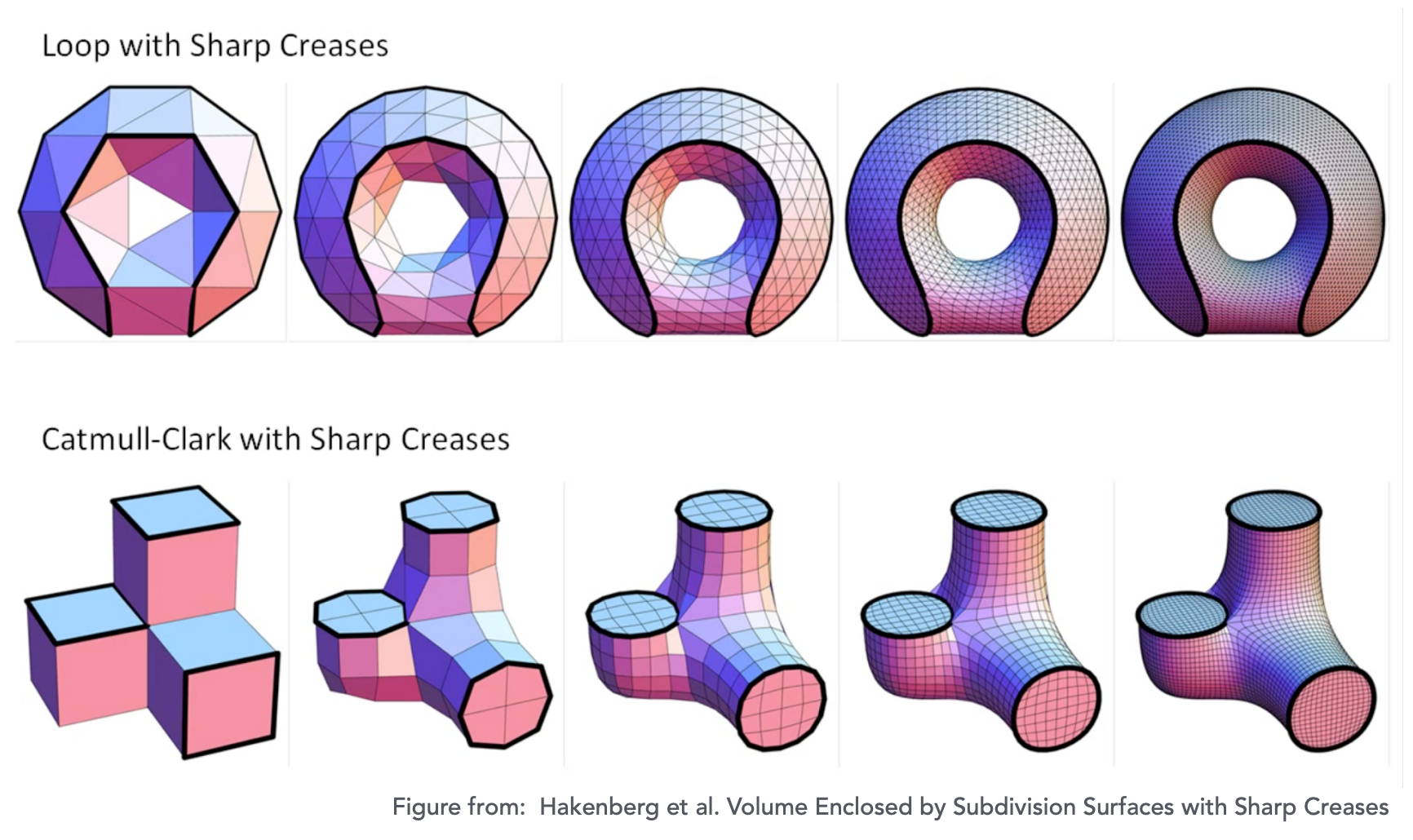
Loop vs Catmull-Clark Subdivision
| Dimension | Loop | Catmull-Clark |
|---|---|---|
| Applicable meshes | Triangle meshes only | General meshes (triangles and quads) |
| Output face type | Triangles | Quads (after the first subdivision) |
| Extraordinary vertices | Introduces no new extraordinary vertices | Introduces extraordinary vertices at the first subdivision, none afterward |
8 Mesh Simplification
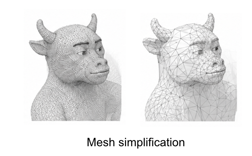
Mesh simplification is a downsampling operation: reduce the number of mesh elements while keeping the overall shape.
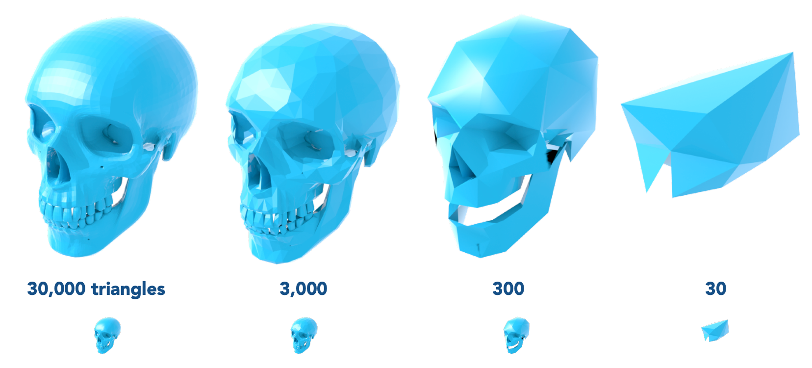
Edge Collapse
Basic idea: simplify meshes by collapsing edges — merge the two endpoints of an edge into a single vertex.
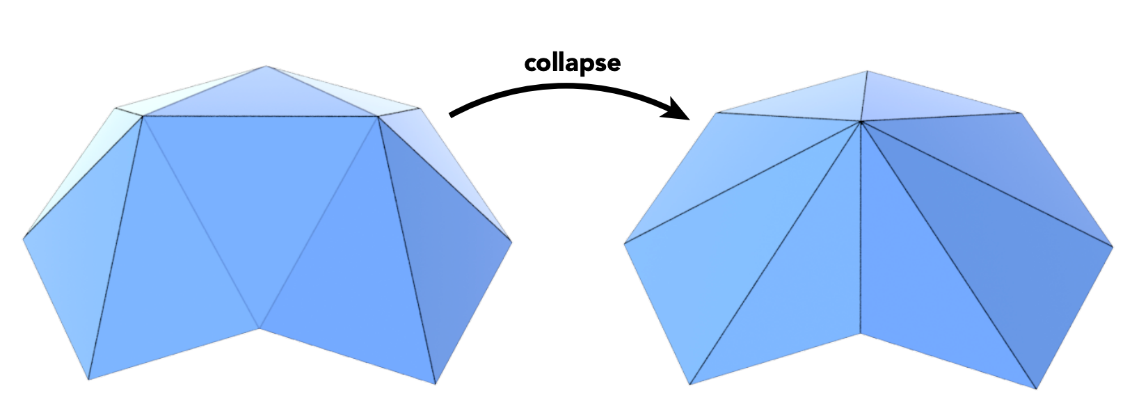
Question: after collapsing an edge, where should the new vertex go?
- Simple approach: take the average of the two endpoints → poor results
- Better approach: use the Quadric Error Metric to pick the optimal position
Quadric Error Metrics (QEM)
Goal: quantify the geometric error introduced by simplification.
Definition: the new vertex should minimize the sum of squared distances (L2 distance) to the planes of the faces it is associated with.
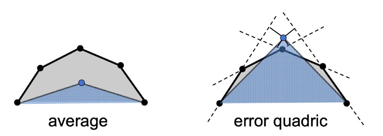
Computation:
- For each edge to be collapsed, compute its quadric error as the cost
- Simple approach: take the edge midpoint and measure its quadric error
- Better approach: pick the position that minimizes the quadric error
Distance approximation: approximate the distance to the surface by the sum of distances to the planes of the containing triangles.
Simplification Algorithm Flow
1. For each edge, compute the quadric error after collapsing (as the edge's "cost")
2. Pick the edge with the smallest cost (smallest quadric error) and collapse it
3. After collapsing, update the quadric errors of affected edges
4. Repeat steps 2-3 until the target face count is reached
This is a greedy algorithm — each step picks the currently best edge to collapse, yet works surprisingly well.
Reference: Garland & Heckbert, 1997. “Surface Simplification Using Quadric Error Metrics”
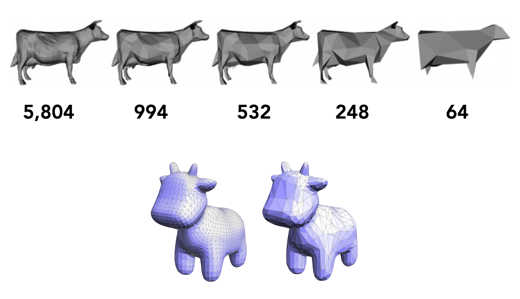
Using a priority queue:
- Sort all edges by quadric error
- Pop the edge with the smallest error and collapse it
- Update the errors of affected edges
- Re-sort
9 Mesh Regularization
Mesh regularization keeps the triangle count unchanged while modifying the sampling distribution to improve mesh quality.
Goal: make triangles closer to equilateral, avoiding thin, over-stretched degenerate triangles.
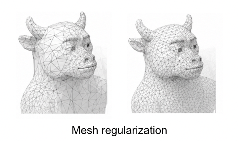
Method:
- Adjust vertex positions so triangle shapes are more uniform
- Do not change the number of triangles or connectivity
- Improves rendering quality and numerical stability
10 Shadow Mapping
Shadow mapping is the classic technique for generating shadows in rasterization — an image-space algorithm.
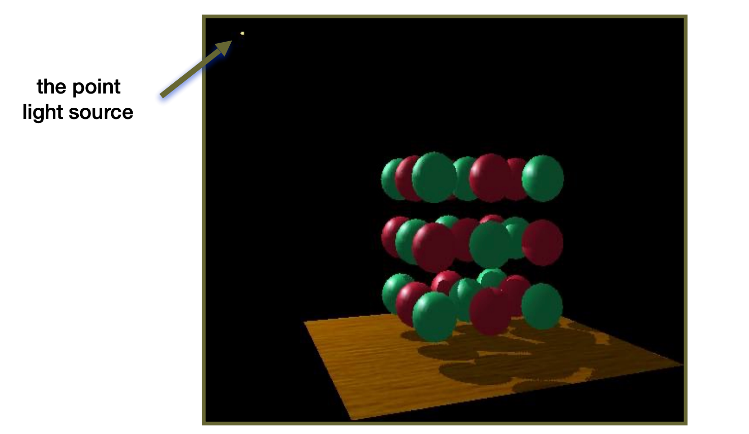
Core Idea
Key observation: a point not in shadow must be seen by both the light and the camera.
If a point:
- Is seen by the camera (visible in the camera view)
- But is not seen by the light (occluded by other objects in the light view)
- Then the point is in shadow
Two-Pass Pipeline
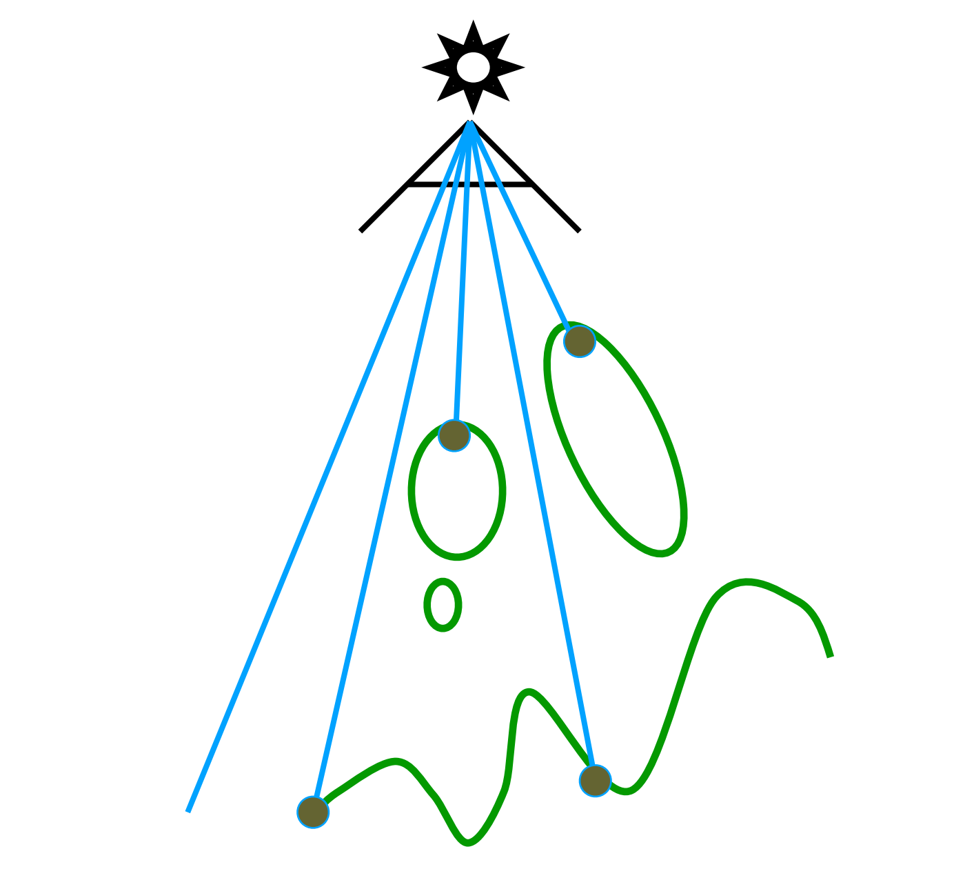
Pass 1: Render from the light
- Put the camera at the light position
- Render the scene, recording only the depth map, not colors
- This depth map is the Shadow Map — it records, from the light’s viewpoint, the closest object distance in every direction
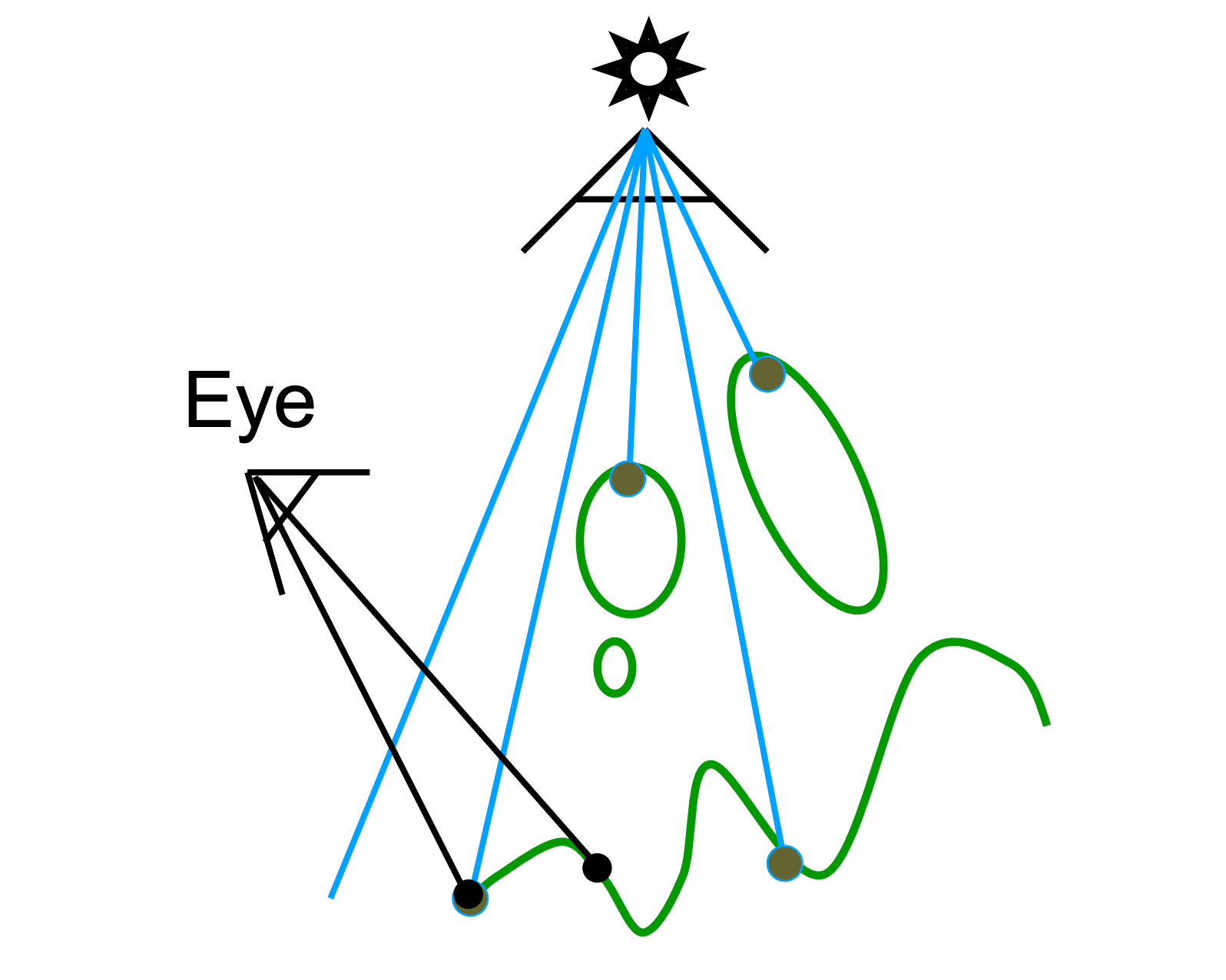
Pass 2A: Render from the eye
- Put the camera back at the original position
- Render the scene normally (with depth) to get the standard image
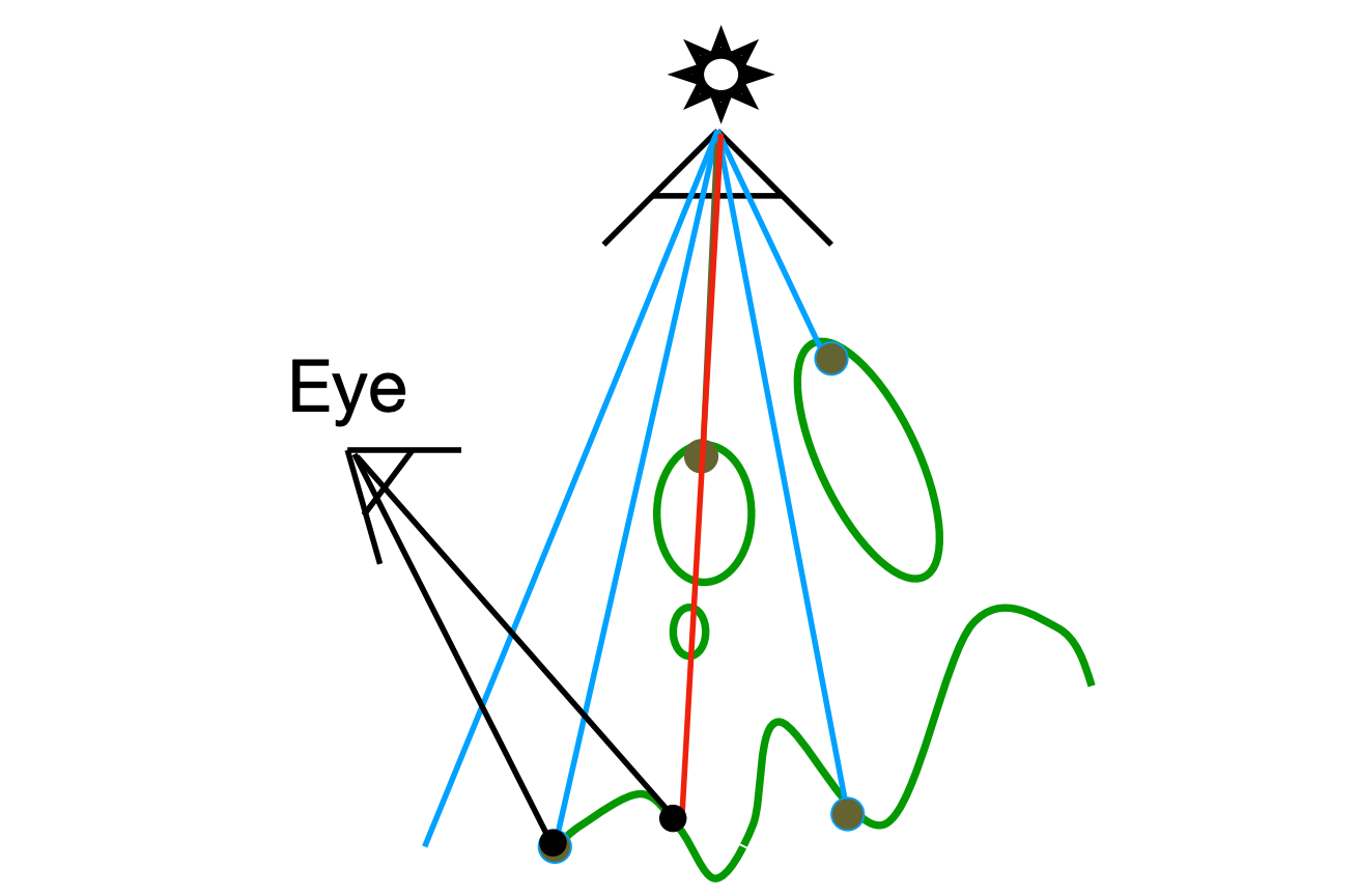
Pass 2B: Project to the light and compare depths
- Re-project every point visible in the camera view back to the light
- Compare the point’s depth with the depth at the corresponding position in the Shadow Map
| Depth comparison | Result | Meaning |
|---|---|---|
| Depths match (approximately equal) | VISIBLE | The point is not occluded — not in shadow |
| Depths mismatch (shadow map depth is smaller) | BLOCKED | The point is in shadow |
Visualization: the depth buffer from the light’s viewpoint (Shadow Map), and comparing Dist(light, shading point) with the shadow map depth at the shading point — green marks regions where depths are approximately equal (visible); non-green is shadow.
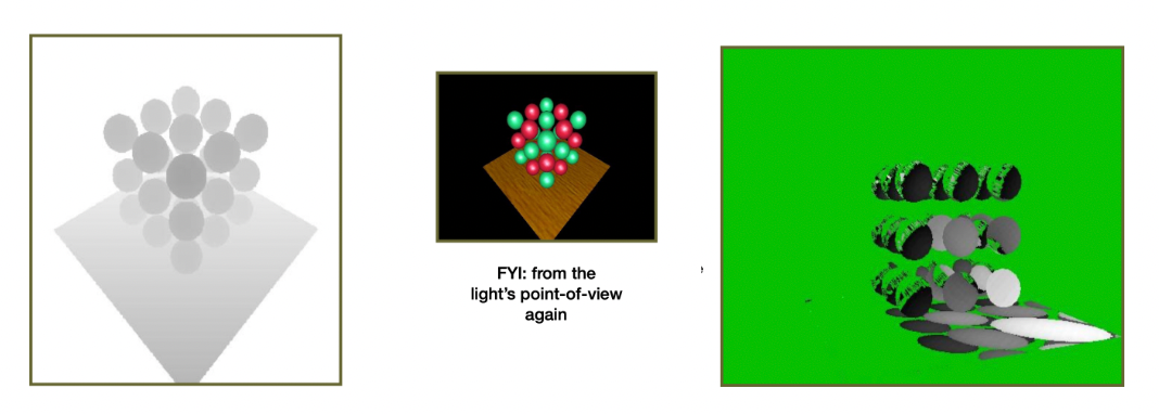
Shadow Mapping Pseudocode
// Pass 1: render from the light
RenderSceneFromLight():
    move the camera to the light position
    render the scene, recording only depth
    obtain shadow_map

// Pass 2: render from the camera
RenderSceneFromEye():
    move the camera to the viewing position
    for each pixel (x, y):
        compute the world position P of the pixel
        project P into the light's view space, get depth d_P
        look up the depth d_shadow at the corresponding position in shadow_map

        if d_P ≈ d_shadow:  // depths match
            the point is not in shadow, shade normally
        else:  // d_P > d_shadow, occluded
            the point is in shadow, skip shading (or darken)
Problems with Shadow Mapping
| Problem | Description |
|---|---|
| Hard shadows | Only produces hard shadows (point lights); no penumbra |
| Resolution dependent | Shadow Map quality depends on its resolution; low resolution leads to jagged shadows |
| Floating-point comparison | Depth comparison involves equality on floats, which has precision issues; needs bias and tolerance handling |
Hard vs Soft Shadows
| Type | Characteristics | Light source |
|---|---|---|
| Hard shadow | Sharp, crisp shadow boundary | Point light |
| Soft shadow | Blurred boundary with penumbra transition | Area light |
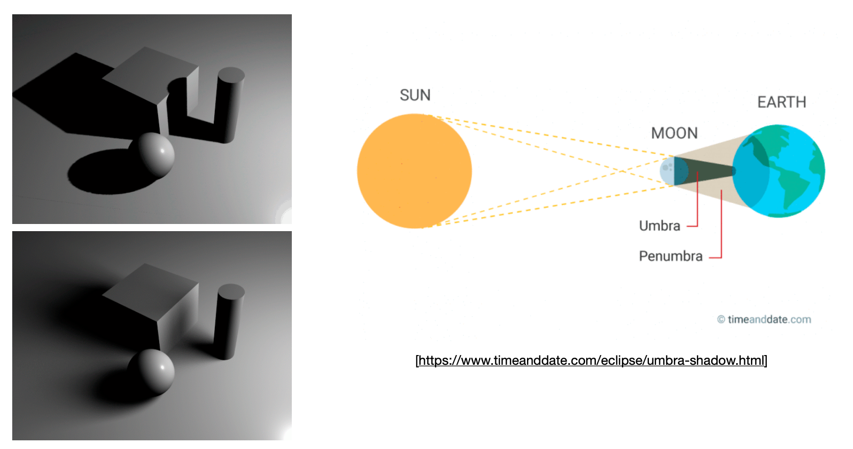
Shadow mapping is a classic rendering technique — it was the fundamental shadow technique of early animated films (e.g. Toy Story) and remains the standard shadow scheme in almost every 3D video game.
Summary
This post covers the core geometry content of GAMES101:
| Topic | Core content |
|---|---|
| Geometry representations | Implicit vs explicit, pros/cons and use cases |
| Implicit geometry | Algebraic surfaces, CSG, distance functions/SDF, level sets, fractals |
| Explicit geometry | Point clouds, polygon meshes, .obj format |
| Bezier curves | de Casteljau algorithm, Bernstein polynomials, properties, piecewise continuity |
| B-splines | Locality advantage; a generalization of Bezier curves |
| Bezier surfaces | $4 \times 4$ control points, separable de Casteljau evaluation |
| Mesh subdivision | Loop subdivision (triangles), Catmull-Clark subdivision (general meshes) |
| Mesh simplification | Edge collapse, quadric error metrics (QEM) |
| Mesh regularization | Keep face count, improve triangle quality |
| Shadow mapping | Two-pass pipeline, depth comparison, hard vs soft shadows |
This post is the 6th note of the GAMES101 - Modern Computer Graphics study series.