- Instructor: Lingqi Yan | UCSB
- Bilibili: https://www.bilibili.com/video/BV1X7411F744
- Lectures covered: Lecture 21 (Animation 1: Basic Concepts, Mass-Spring Systems, Kinematics, Rigging / Blend Shapes / Motion Capture), Lecture 22 (Animation Cont.: Solving ODEs, Rigid Body and Fluids)
Note: the previous eleven posts all dealt with the “static” problem — a scene sits there, and we care about how to compute and draw it. This one changes the dimension: making the scene move over time. Animation and simulation both look like they “generate motion”, but they take two fundamentally different routes: animation describes motion (a human supplies keyframes or joint angles and the computer interpolates), while simulation derives motion (a human supplies the laws of physics and the computer integrates). In practice the two roads meet in the same place — both end up solving differential equations numerically, and both can blow up because of discretisation.
1 Animation Basics
Animation is “bringing things to life”. It is at once a communication tool (conveying visual information) and an extension of modelling (expressing a scene model as a function of time), and it outputs a sequence of images that produce a sensation of motion when viewed in order.
Frame rates for different applications
| Application | Frame rate (fps) | Note |
|---|---|---|
| Film | 24 fps | The classic cinema standard |
| Video | 30 fps | The general video standard |
| Virtual reality (VR) | 90 fps | The high frame rate prevents nausea |
A brief history of animation
| Year | Event | Significance |
|---|---|---|
| 3200 BCE | Iranian pottery bowl animation | The earliest known animation |
| 1831 | Phenakistoscope | An early animation device |
| 1878 | Muybridge, “Sallie Gardner” | The first film (a scientific tool) |
| 1937 | Disney’s Snow White | The first feature-length hand-drawn animated film |
| 1963 | Sutherland’s “Sketchpad” | The first computer-generated animation |
| 1972 | Catmull & Parke’s computer face | Early computer animation |
| 1993 | Jurassic Park | Digital dinosaurs |
| 1995 | Pixar’s Toy Story | The first CG feature film |
| 2009 | Sony’s Cloudy with a Chance of Meatballs | The state of CG animation a decade earlier |
| 2019 | Disney’s Frozen 2 | The state of CG animation in 2019 |
The table is really a very direct Moore’s-law-style observation: the technical gap between consecutive rows is roughly proportional to the time gap, and it took thirty years to go from Sketchpad in 1963 to Toy Story in 1995, but only twenty-four to go from 1995 to 2019.
Keyframe animation
The core idea is to split the production of animation into two layers:
- Keyframes: the important frames created by the lead animator
- Tweens: the in-between frames generated automatically by assistants or the computer (“tweening”)
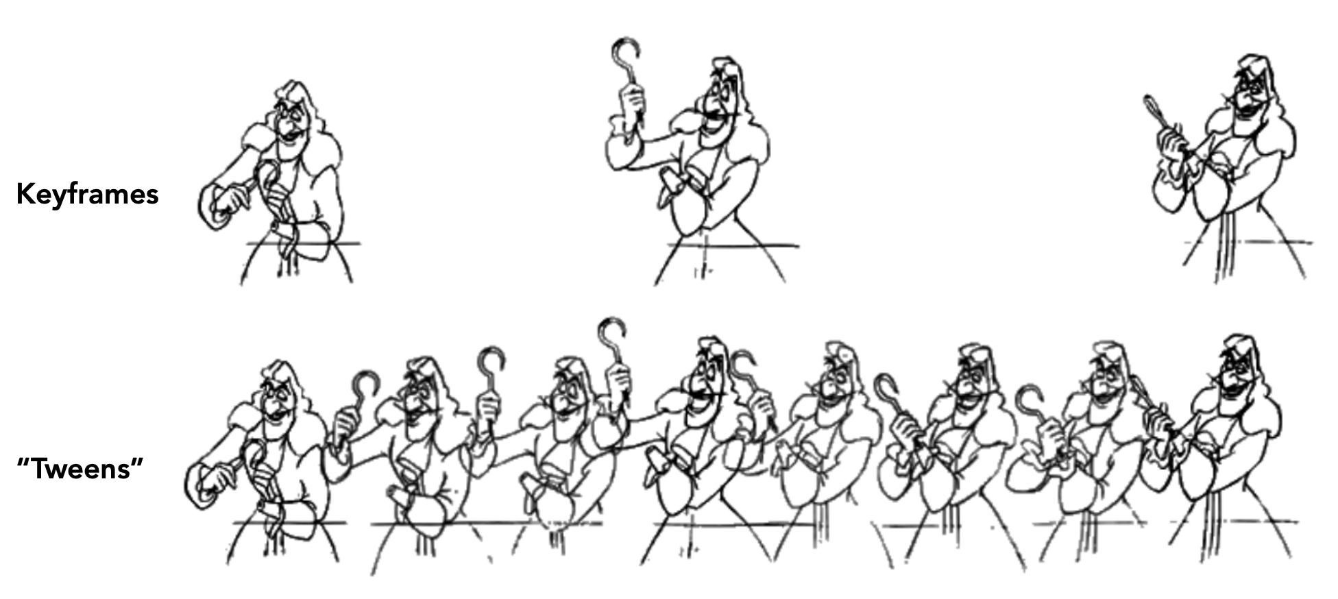
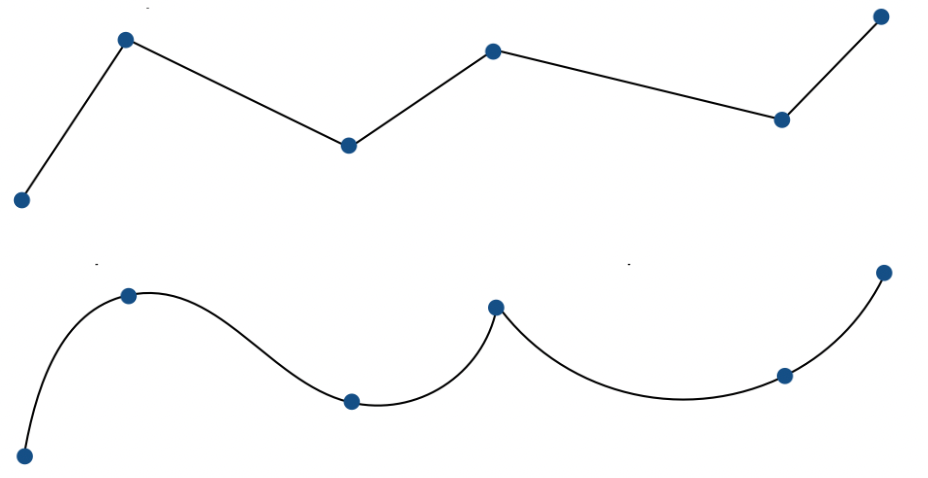
Keyframe interpolation treats every frame as a vector of parameter values and interpolates each parameter separately. Linear interpolation is usually not good enough; you want splines, for smooth and controllable interpolation.
Physical simulation
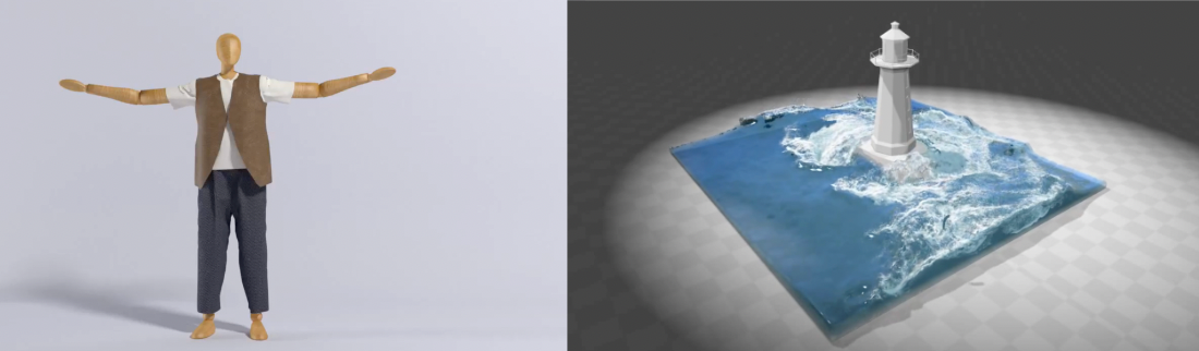
Physical simulation starts from Newton’s law:
$$ \mathbf{F} = m\mathbf{a} $$where $\mathbf{F}$ is force, $m$ is mass and $\mathbf{a}$ is acceleration. Physics-based animation uses numerical simulation to generate motion, for example extrapolating the next state from the current one:
$$ \mathbf{x}^{t+\Delta t} = \mathbf{x}^{t} + \Delta t \, \mathbf{v}^{t} + \frac{1}{2}(\Delta t)^2 \mathbf{a}^{t} $$There are three classic application areas:
| Application | Note |
|---|---|
| Cloth simulation | Modelling fabric with mass-spring systems |
| Fluid simulation | Simulating water, smoke and similar effects |
| Ropes / hair | Chain of springs or a particle system |
2 Mass Spring Systems
The mass-spring system is the classic way to model dynamic systems: connect point masses with springs to simulate cloth, ropes, hair and more. It is probably the highest return-on-investment simulation method in all of graphics — one principle, Hooke’s law, yet it supports cloth, hair and soft bodies across a huge range of applications.
Dot notation
Let $\mathbf{x}$ be the position vector of a point; a dot denotes the derivative with respect to time:
| Symbol | Meaning | Relation |
|---|---|---|
| $\mathbf{x}$ | Position | — |
| $\dot{\mathbf{x}}$ | Velocity $\mathbf{v}$ | First derivative of position w.r.t. time |
| $\ddot{\mathbf{x}}$ | Acceleration $\mathbf{a}$ | Second derivative of position w.r.t. time |
The ideal spring (Hooke’s law)
With two endpoints $a$ and $b$, the spring pulls the two points together, with force proportional to displacement (Hooke’s law):
$$ \mathbf{f}_{a \to b} = k_s(\mathbf{b} - \mathbf{a}) $$$$ \mathbf{f}_{b \to a} = -\mathbf{f}_{a \to b} $$where $k_s$ is the spring constant (stiffness).
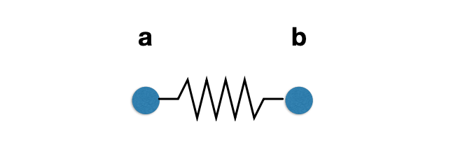
Problem: an ideal spring has zero rest length, so it keeps pulling the two points until they coincide.
The non-zero length spring
Introduce a rest length $l$; the spring exerts no force when its length equals $l$:
$$ \mathbf{f}_{a \to b} = k_s \frac{\mathbf{b} - \mathbf{a}}{\|\mathbf{b} - \mathbf{a}\|} \left( \|\mathbf{b} - \mathbf{a}\| - l \right) $$Break the formula into three parts:
| Part | Meaning |
|---|---|
| $\frac{\mathbf{b} - \mathbf{a}}{\|\mathbf{b} - \mathbf{a}\|}$ | Unit direction vector pointing from $a$ to $b$ |
| $\|\mathbf{b} - \mathbf{a}\| - l$ | Difference between current length and rest length (a scalar) |
| $k_s$ | Spring stiffness coefficient |
Problem: such a spring oscillates forever (no energy is lost), so damping is needed.
Internal damping
The naive idea is to add a drag proportional to velocity:
$$ \mathbf{f} = -k_d \dot{\mathbf{b}} $$This is like viscous drag, but it slows down all motion (including global translation and rotation) — whereas we only want to damp the internal motion driven by the spring, not have the whole object fall more slowly.
Internal spring damping applies viscous drag only along the direction of the spring’s length change:
$$ \mathbf{f}_{a \to b} = -k_d \left( \frac{\mathbf{b} - \mathbf{a}}{\|\mathbf{b} - \mathbf{a}\|} \cdot (\dot{\mathbf{b}} - \dot{\mathbf{a}}) \right) \frac{\mathbf{b} - \mathbf{a}}{\|\mathbf{b} - \mathbf{a}\|} $$Key points:
- The damping force acts only along the direction in which the spring’s length changes
- It does not slow down the overall motion of the spring system (global translation or rotation)
- $k_d$ is the damping coefficient
This expression deserves a second look: $\frac{\mathbf{b}-\mathbf{a}}{\|\mathbf{b}-\mathbf{a}\|}$ is the unit vector along the spring axis and $(\dot{\mathbf{b}}-\dot{\mathbf{a}})$ is the relative velocity of the two endpoints. The dot product of the two extracts the component of the relative velocity along the spring axis; multiplying back by the unit vector turns that scalar back into a force along the axis. Any relative velocity perpendicular to the spring (i.e. overall rotation) is filtered out by the dot product directly — which is exactly the mechanism that damps only internal deformation.
Structures from springs
By use, spring structures fall into three categories: sheets (planar, like cloth), blocks (volumetric, like 3D solids) and others (ropes, chains).
Spring behaviour is determined by its connection structure, and different structures have different physical properties:
| Structure | Shear resistance | Bending resistance | Characteristics |
|---|---|---|---|
| Structure 1 (horizontal/vertical only) | No | No | Cannot resist shear or out-of-plane bending |
| Structure 2 (with diagonals) | Yes (anisotropic) | No | Resists shear, but with directional bias |
| Structure 3 (both diagonals) | Yes (less bias) | No | More uniform shear resistance, still no bending resistance |
| Structure 4 (with jump connections) | Yes | Yes | Complete structure; the red jump springs must be much weaker |
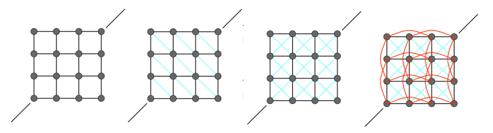
Correspondingly there are three spring types:
- Structural springs: horizontal/vertical connections, maintaining the basic shape
- Shear springs: diagonal connections, resisting shear deformation
- Bending springs: jump connections (skipping one point mass), resisting out-of-plane bending, with stiffness far lower than the other two
That last point is easy to miss: bending springs span a longer distance, so if their stiffness matched the structural springs the cloth would be stiff as sheet metal. It is precisely because they must be far weaker that they are drawn in a “secondary” colour like red in the structural diagram.
Applications
| Application | Note |
|---|---|
| Ropes | A chain of point masses and springs |
| Hair | A chain of springs modelling strands |
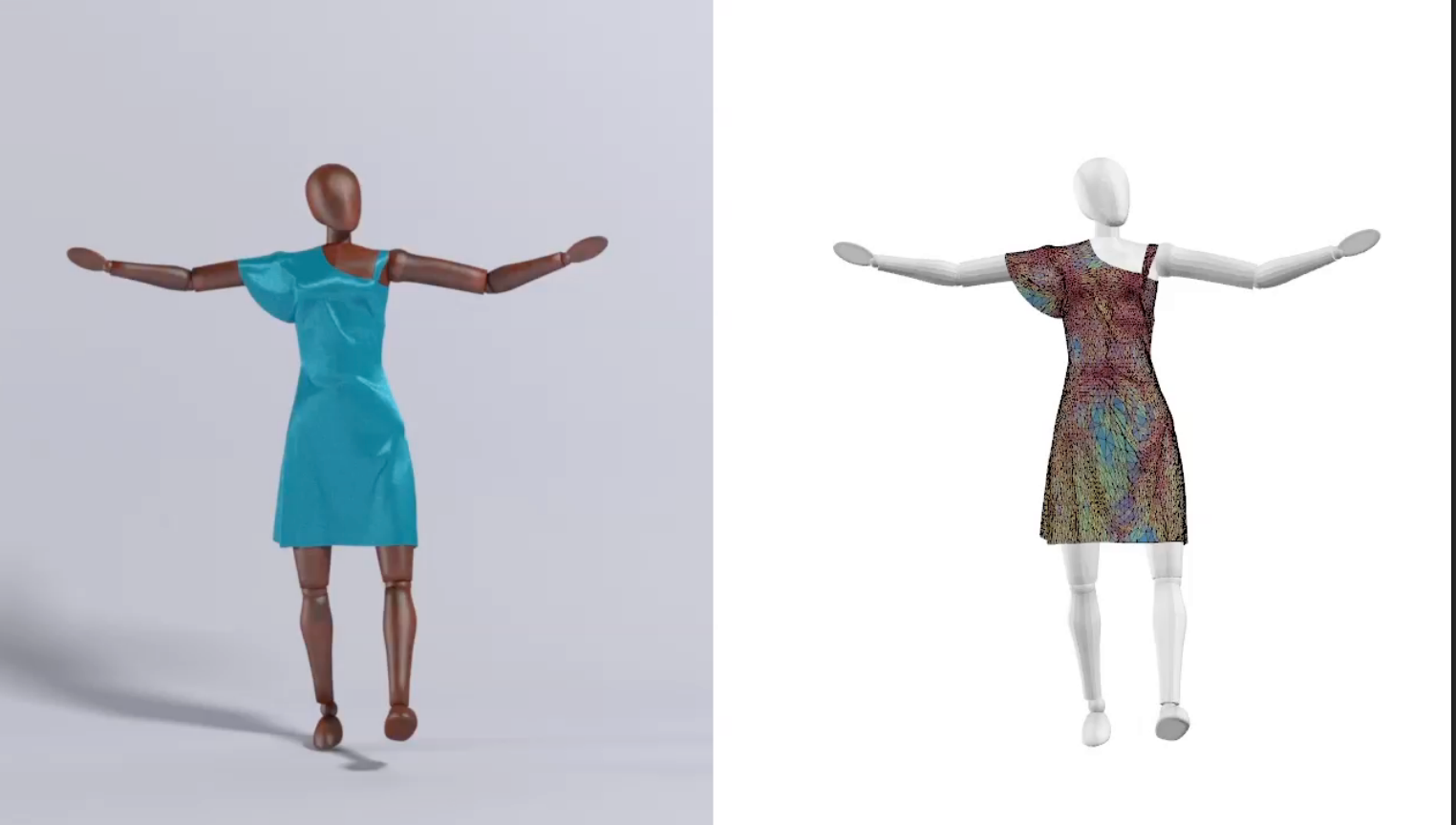
| Cloth mesh | A mass-spring grid modelling fabric, optionally combined with data-driven elastic models |
| Dress + character | Combined simulation of a spring-based dress colliding with a character’s body |
The finite element method (FEM)
Besides spring systems, one can use the finite element method (FEM) to simulate elastic bodies. FEM discretises a continuum into finitely many elements and solves the partial differential equations directly; it is more accurate than mass-spring systems, but also more computationally demanding.
3 Particle Systems
Basic concepts
A particle system models a dynamic system as a large collection of particles, each moving under a set of physical (or non-physical) forces.
Advantages:
- Easy to understand and implement
- Scalable: few particles are fast, many particles are detailed
Challenges:
- May require a great many particles (e.g. fluids)
- May require acceleration structures (e.g. to find neighbouring particles for interaction)
The particle system algorithm
The update loop for each frame of animation:
For each frame in animation:
    1. [If needed] Create new particles
    2. Compute the forces on each particle
    3. Update position and velocity of each particle
    4. [If needed] Remove dead particles
    5. Render the particles
Note that “create” and “remove” are optional — and it is exactly that optionality that lets particle systems express phenomena with a life cycle, like flames, smoke and spray: particles are emitted, survive some number of frames, then disappear.
Forces on particles
| Force type | Example |
|---|---|
| Attraction / repulsion | Gravity, electromagnetic force |
| Spring / propulsion | Spring connections, thrusters |
| Damping | Friction, air drag, viscosity |
| Collision | Walls, containers, fixed objects, dynamic objects, character body parts |
Gravitational attraction
The attraction between particles follows Newton’s law of universal gravitation:
$$ F_g = G \frac{m_1 m_2}{d^2} $$where:
- $G = 6.67428 \times 10^{-11} \, \text{N}\cdot\text{m}^2\cdot\text{kg}^{-2}$ (the gravitational constant)
- $m_1, m_2$ are the masses of the two particles
- $d$ is the distance between them
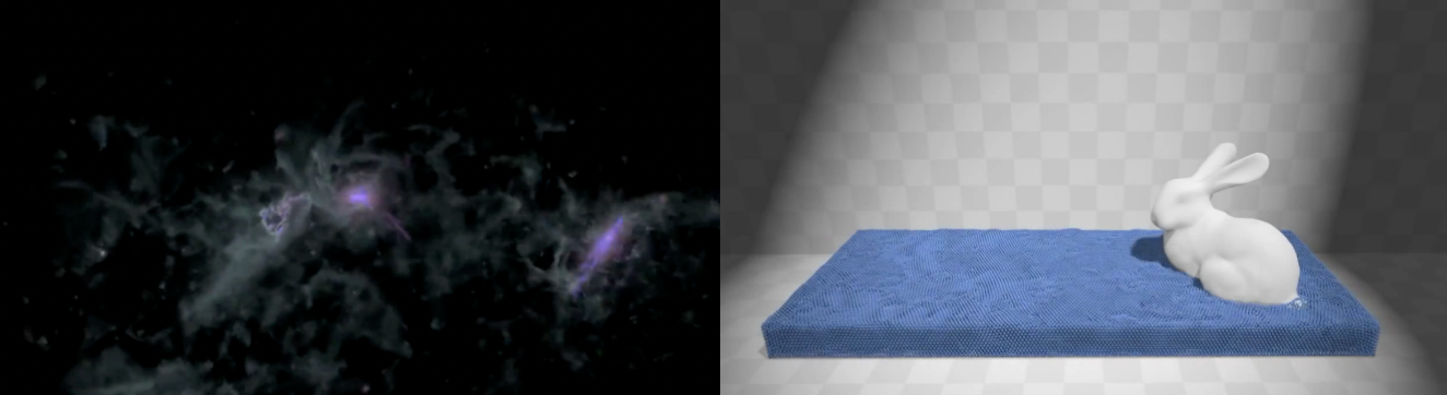
Application: galaxy simulation (disc galaxy simulation, NASA Goddard).
Simulated flocking
Model each bird as a particle under simple forces, and numerically evolve a large particle system to obtain emergent complex behaviour:
| Force | Effect |
|---|---|
| Attraction | Pull towards the centre of neighbouring birds |
| Repulsion | Move away from neighbours that are too close |
| Alignment | Turn towards the average direction of neighbours |
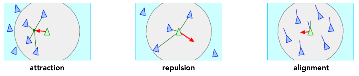
Each of these three forces is extremely simple on its own, yet together they produce “a flock” — a global behaviour nobody designed explicitly. The same emergent behaviour is observed in nature with schools of fish and swarms of bees.
Further applications
- Position Based Fluids: Macklin and Müller simulate incompressible water with many particles plus density constraints
- Molecular dynamics: an ice-crystal melting model showing ice turning to water through inter-particle interaction
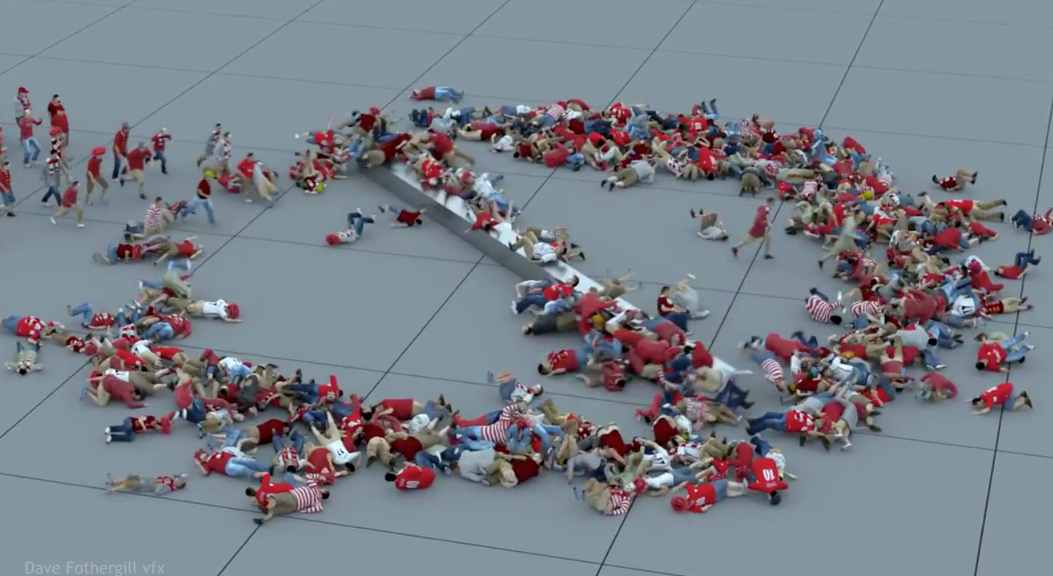
- Crowd simulation: Crowds + “Rock” Dynamics, large-scale crowds combined with “rock concert” dynamics
4 Kinematics
Articulated skeleton
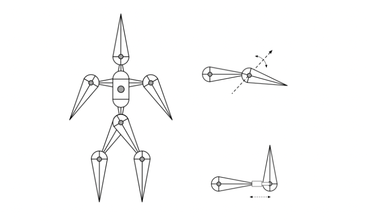
A skeleton is described by three things:
- Topology: what connects to what (a tree structure when acyclic)
- Geometry: defined by the joints
- Joint types:
| Joint type | DOF | Note |
|---|---|---|
| Pin | 1D rotation | Rotates about an axis |
| Ball | 2D rotation | Rotates in any direction |
| Prismatic | Translation | Slides along an axis |
Forward kinematics
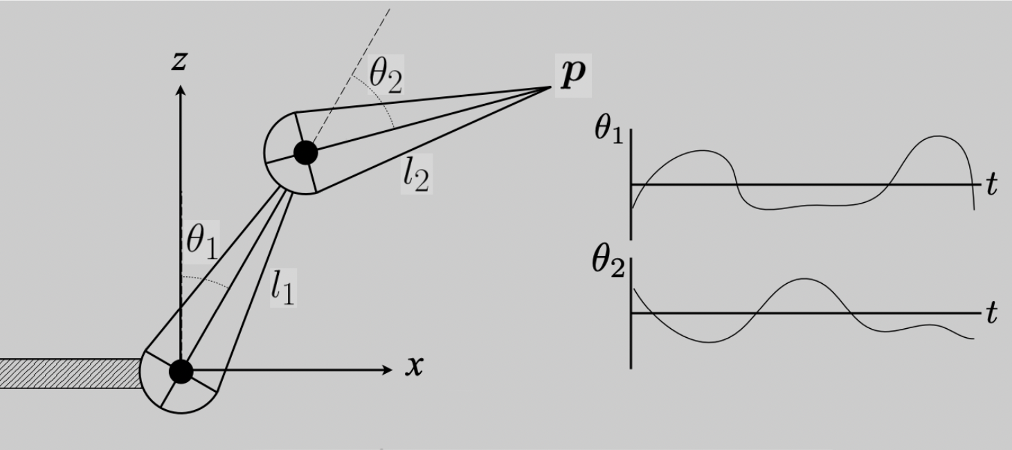
Core idea: the animator supplies joint angles, and the computer determines the position of the end effector.
Take a 2D two-segment arm as an example (note: this is a Z-up coordinate system):
$$ p_x = l_1 \sin(\theta_1) + l_2 \sin(\theta_1 + \theta_2) $$$$ p_z = l_1 \cos(\theta_1) + l_2 \cos(\theta_1 + \theta_2) $$where $l_1, l_2$ are the lengths of the two segments and $\theta_1, \theta_2$ are the joint angles. The animation is then simply these angles written as functions of time.
| Advantages | Disadvantages |
|---|---|
| Direct control, convenient | Motion may be physically inconsistent |
| Simple to implement | Time-consuming for the animator |
This “Z-up” premise matters: because $\theta$ is measured from the Z axis, the first segment’s components are $(\sin\theta_1, \cos\theta_1)$ rather than the more familiar $(\cos\theta_1, \sin\theta_1)$. Copying the habitual form would lay the whole skeleton on its side.
Inverse kinematics
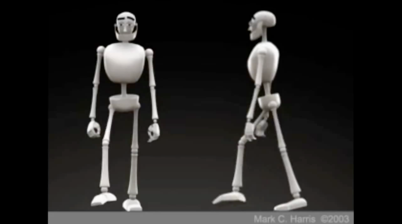
Core idea: the animator supplies the position of the end effector, and the computer must determine joint angles that satisfy the constraint — exactly the reverse of forward kinematics.
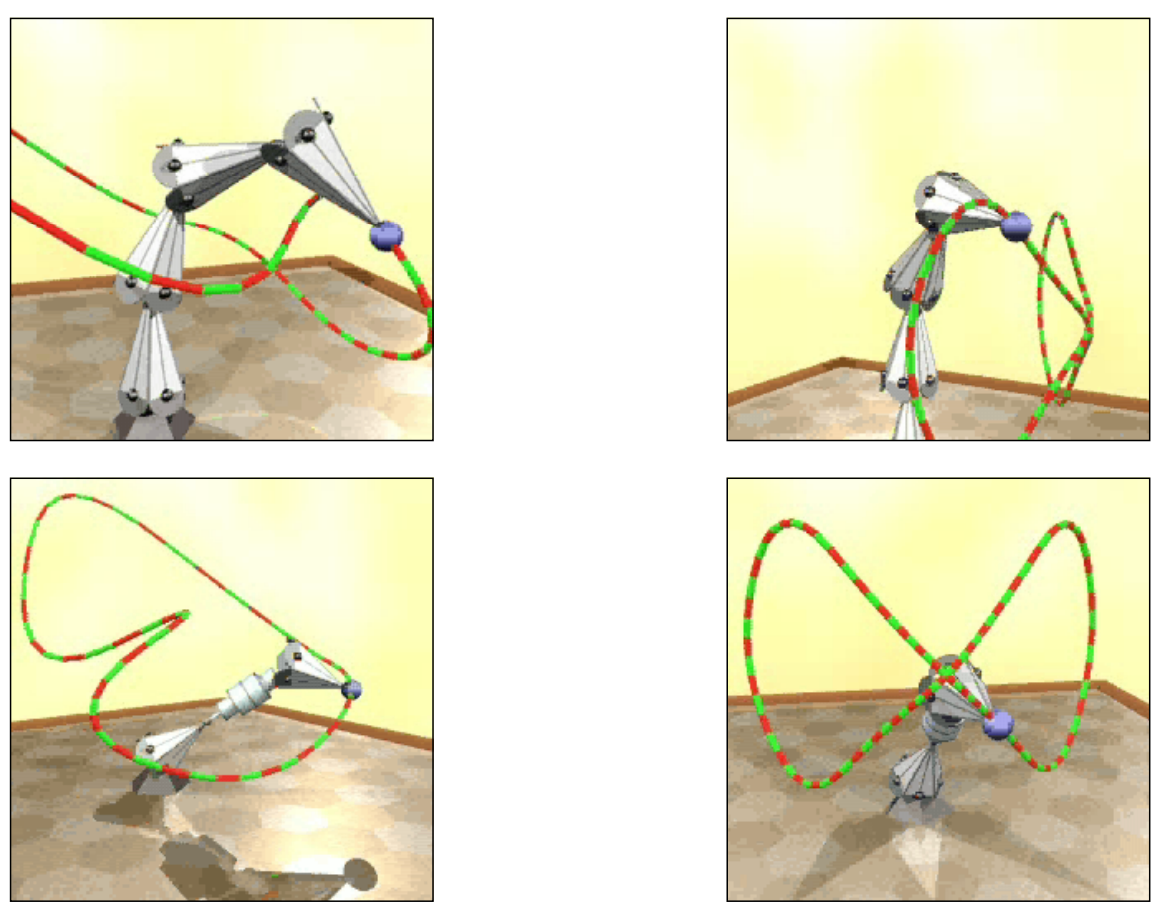
Analytic solution (two-segment arm): for a simple structure like a two-segment arm one can solve analytically. By the law of cosines:
$$ \theta_2 = \cos^{-1}\left(\frac{p_z^2 + p_x^2 - l_1^2 - l_2^2}{2 \, l_1 \, l_2}\right) $$Numerical solutions: for more complex skeletons an analytic solution is usually impossible, so numerical methods are needed (gradient descent, Jacobian-based iterations, etc.).
| Method | Suitable for |
|---|---|
| Analytic | Simple structures (e.g. a two-segment arm) |
| Numerical | Complex structures, general purpose |
Difficulties of IK:
- Multiple solutions may exist
- There may be no solution (unreachable target)
- Numerical methods may converge to a local optimum
That $\cos^{-1}$ form already hints at the first difficulty: $\theta_2$ and $-\theta_2$ give the same cosine, corresponding to “elbow up” and “elbow down” — two different poses, and the computer has no way to choose. Disambiguation usually requires extra constraints such as joint angle limits.
Style-based IK
Style-based inverse kinematics (Grochow et al., Style Based Inverse Kinematics, 2004) solves IK not in the raw joint space but in a pose space learned from data, so that the solution matches a particular character’s style of movement. “Does this look like this person?” becomes part of the solving constraints.
Rigging
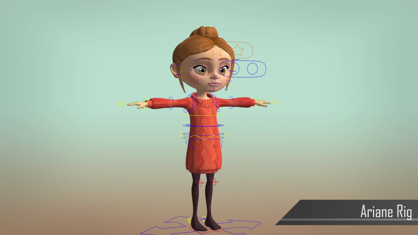
Rigging is a set of high-level controls on a character, used to modify pose, deformation and expression more quickly and intuitively.
| Point | Note |
|---|---|
| Analogy | Like the strings on a marionette |
| Coverage | Should capture all meaningful character variation |
| Character-specific | Each character needs its own rig |
| Cost of creation | High — purely manual, requiring training in both art and technology |
Blend shapes
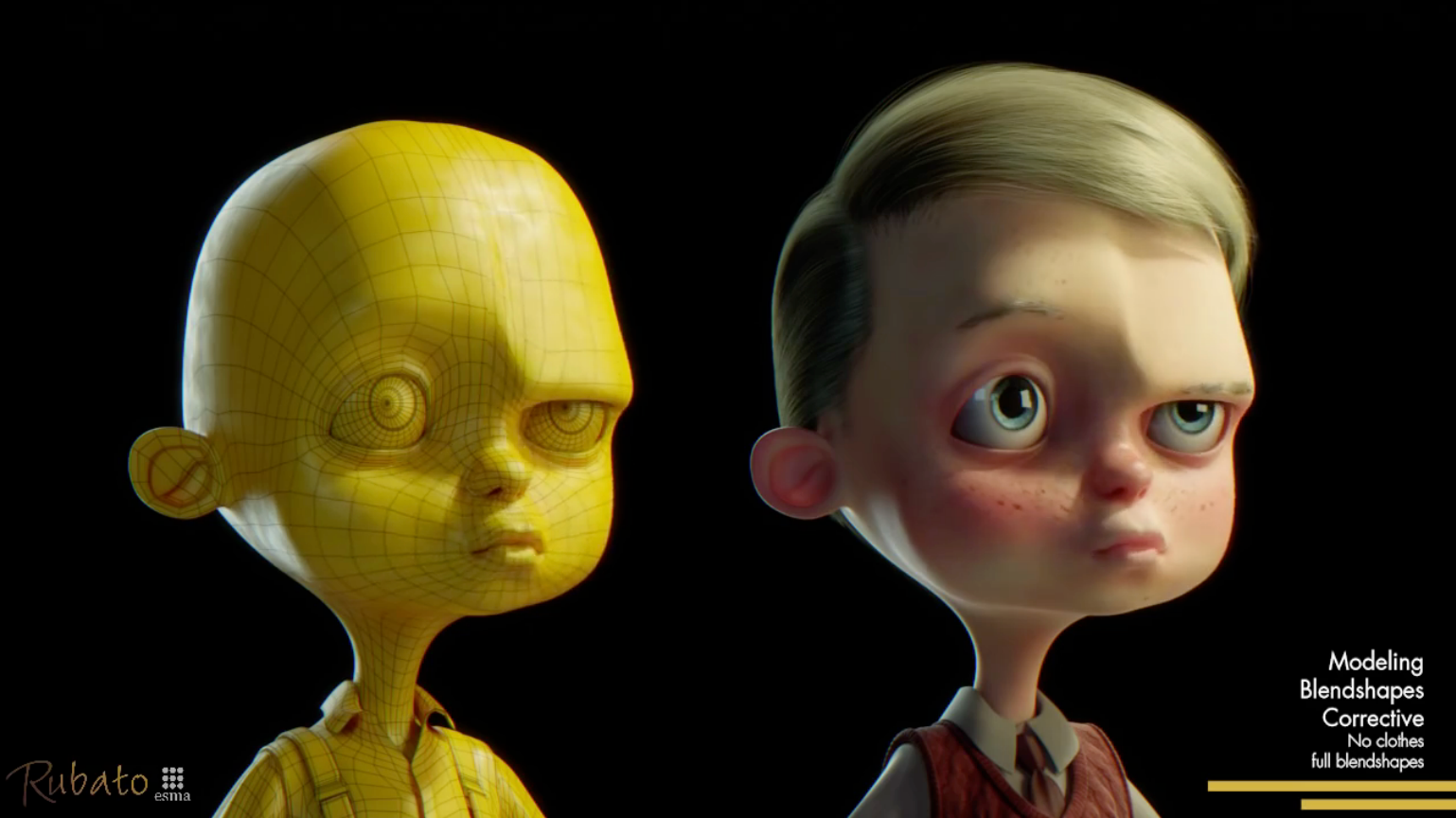
Blend shapes do not use a skeleton; they interpolate directly between different surfaces:
- Typical use: model a set of facial expressions and interpolate directly between the expression surfaces
- Simplest scheme: a linear combination of the corresponding vertex positions
- Weight control: weights can be driven over time by splines
Motion capture
Definition: a data-driven approach to creating animation — record a real-world performance (say, a person carrying out an activity) and extract the variation of pose over time from the captured data.
| Advantages | Disadvantages |
|---|---|
| Captures a large amount of real data quickly | Complex, expensive equipment |
| Can achieve high realism | The captured animation may not fit the artistic need and requires reworking |
Three classes of device:
| Type | Principle | Characteristics |
|---|---|---|
| Optical | Retroreflective markers + infrared cameras | The mainstream approach, high accuracy |
| Magnetic | Infer position/orientation from induced magnetic fields | Requires being tethered |
| Mechanical | Measure joint angles directly | Restricts movement |
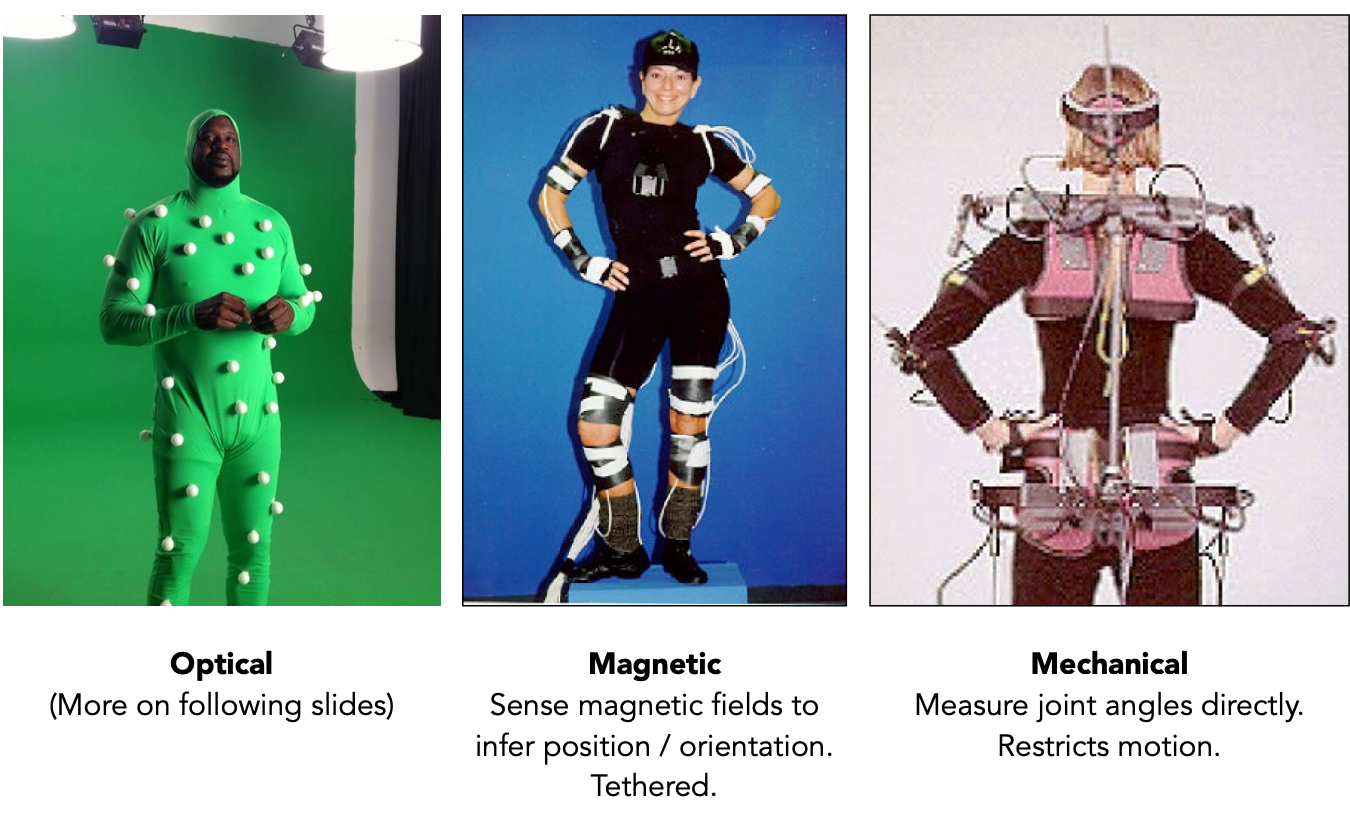
Optical motion capture in detail:
- Retroreflective markers are attached to the performer
- Combined with infrared lighting and infrared cameras
- Positions are determined by triangulation across multiple cameras
- Typically eight or more cameras, at 240 Hz
- Occlusions are hard to handle
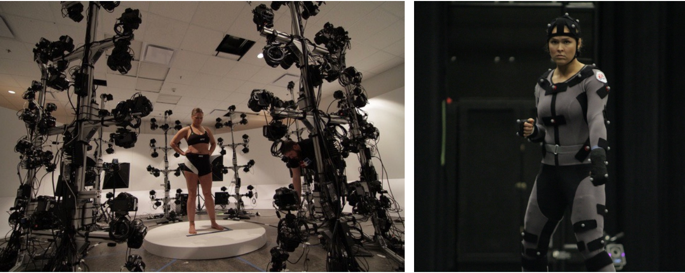
Extracting motion data is not a trivial task: a single subset of the motion curves extracted from a captured walk already shows how involved it is (Witkin and Popovic, 1995) — there is a great deal of work between a point cloud and a usable action.
The uncanny valley: in robotics and graphics, when an artificial character’s appearance approaches human realism, the audience’s emotional response actually gets worse, until the character’s expressiveness becomes convincing enough. The lecture contrasts cartoon style (Brave, Pixar) with semi-realistic style (The Polar Express, Warner Bros.).
Facial motion capture: Avatar mapped facial capture from the actor onto the virtual character.
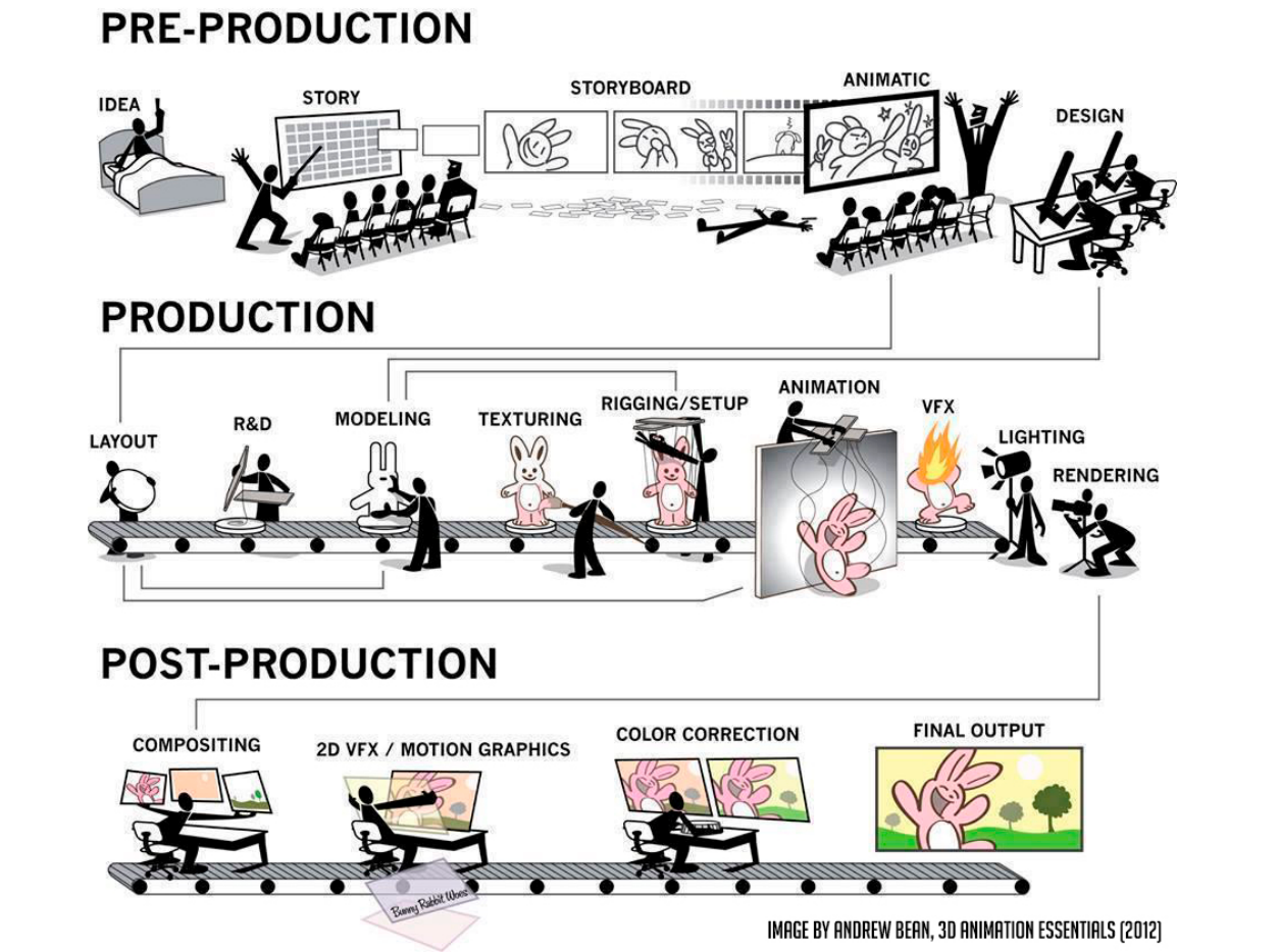
The production pipeline
The industrial pipeline for a whole animation is: first modelling, then rigging, then generate motion through animation and simulation, and finally rendering to produce the finished result.
5 Solving ODEs
Single particle simulation
Start with the motion of a single particle, then generalise to many.
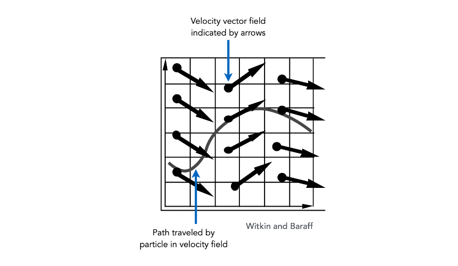
Suppose a particle’s motion is determined by a velocity vector field $\mathbf{v}(\mathbf{x}, t)$ (a function of position and time). Computing the particle’s position over time means solving a first-order ordinary differential equation (ODE):
$$ \frac{d\mathbf{x}}{dt} = \dot{\mathbf{x}} = \mathbf{v}(\mathbf{x}, t) $$- “First-order”: only first derivatives appear
- “Ordinary”: no partial derivatives — $\mathbf{x}$ is a function of $t$ alone
Given an initial position $\mathbf{x}_0$, we solve by forward numerical integration.
Explicit Euler (forward Euler)
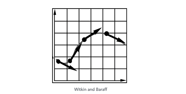
Method: a simple iterative method; commonly used but inaccurate, and unstable in most cases.
$$ \mathbf{x}^{t+\Delta t} = \mathbf{x}^{t} + \Delta t \, \dot{\mathbf{x}}^{t} $$$$ \dot{\mathbf{x}}^{t+\Delta t} = \dot{\mathbf{x}}^{t} + \Delta t \, \ddot{\mathbf{x}}^{t} $$That is, extrapolate the next position and velocity directly from the current velocity and acceleration.
Errors and instability
Numerical integration with finite differences introduces two problems:
1. Errors:
- Error accumulates at every time step
- Accuracy degrades as the simulation proceeds
- In graphics applications accuracy may not be the critical concern
2. Instability:
- Errors can compound, causing the simulation to diverge (even when the underlying system does not)
- Instability is a fundamental problem in simulation and cannot be ignored
- A catastrophic example: vehicles in PUBG diverging because of numerical instability
Source of error: the larger the time step $\Delta t$, the larger the error and the more likely divergence becomes.
Explicit Euler is simple but low-order (first-order), and prone to instability on stiff equations and oscillatory systems. Physical simulation commonly uses semi-implicit Euler or Verlet instead, while stiff scenes require implicit methods.
Ways to fight instability
| Method | Core idea |
|---|---|
| Midpoint method / modified Euler | Average the velocity at the start and the end |
| Adaptive step size | Compare one step against two half steps, recursing until the error is acceptable |
| Implicit methods | Use the velocity at the next time step (harder but more stable) |
| Position-based / Verlet integration | Constrain particle positions and velocities after the time step |
Midpoint method
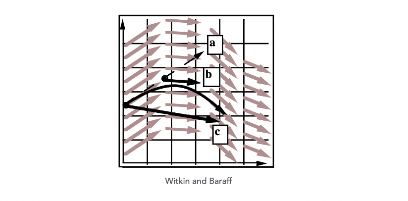
Steps:
- Extend the original position and take an Euler step (giving an intermediate predicted position)
- Evaluate the derivative at the midpoint
- Update the position using the midpoint derivative
Modified Euler
Averaging the velocities at the start and the end of the step works even better:
$$ \mathbf{x}^{t+\Delta t} = \mathbf{x}^{t} + \frac{\Delta t}{2}\left(\dot{\mathbf{x}}^{t} + \dot{\mathbf{x}}^{t+\Delta t}\right) $$$$ \dot{\mathbf{x}}^{t+\Delta t} = \dot{\mathbf{x}}^{t} + \Delta t \, \ddot{\mathbf{x}}^{t} $$Substituting and eliminating gives:
$$ \mathbf{x}^{t+\Delta t} = \mathbf{x}^{t} + \Delta t \, \dot{\mathbf{x}}^{t} + \frac{(\Delta t)^2}{2} \ddot{\mathbf{x}}^{t} $$which agrees exactly with the displacement formula for uniform acceleration in physics.
Adaptive step size
Adaptive step size chooses the step from an error estimate; it is very practical but may need a very small step.
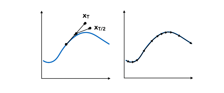
Algorithm:
Repeat until the error is below the threshold:
    1. Take an Euler step of size T to compute x_T
    2. Take two Euler steps of size T/2 to compute x_{T/2}
    3. Compute the error ||x_T - x_{T/2}||
    4. If the error > threshold, reduce the step and retry
Advantage: automatically adapts to the accuracy needed in different regions.
Disadvantage: may require extremely small steps, making the cost unpredictable.
Implicit Euler (backward Euler)
Implicit Euler updates the state using the derivative at the next moment, so it requires solving an implicit equation. Its accuracy is only first-order, but it is unconditionally stable, which makes it especially suitable for stiff equations and for scenes that need large steps. The only difference from explicit Euler is that it uses the derivative at the next moment rather than the current one.
$$ \mathbf{x}^{t+\Delta t} = \mathbf{x}^{t} + \Delta t \, \dot{\mathbf{x}}^{t+\Delta t} $$$$ \dot{\mathbf{x}}^{t+\Delta t} = \dot{\mathbf{x}}^{t} + \Delta t \, \ddot{\mathbf{x}}^{t+\Delta t} $$How to solve: you need to solve a nonlinear system in $\mathbf{x}^{t+\Delta t}$ and $\dot{\mathbf{x}}^{t+\Delta t}$, typically with a root-finding algorithm such as Newton’s method.
Stability analysis: use the local truncation error (per step) and the total accumulated error (overall) to measure stability:
| Error type | Implicit Euler |
|---|---|
| Local truncation error | $O(h^2)$ |
| Global truncation error | $O(h)$ |
where $h$ is the step size (that is, $\Delta t$). What $O(h)$ means: halve the step and the error roughly halves too.
Explicit and implicit form a very typical trade-off here: each step of an implicit method is far more expensive (you must solve a nonlinear system), but it permits a far larger step; each step of an explicit method is cheap, but it blows up as soon as the step grows. Which one to pick in practice depends on how “stiff” the problem is.
Runge-Kutta methods (RK4)
The classical fourth-order Runge-Kutta method (RK4) is one of the most widely used methods for solving ODEs numerically. By evaluating four slopes within a single step and taking a weighted average, it reaches fourth-order accuracy and strikes an excellent balance between accuracy, stability and cost, excelling particularly on nonlinear problems.
Initial condition:
$$ \frac{dy}{dt} = f(t, y), \quad y(t_0) = y_0 $$The RK4 solution:
$$ y_{n+1} = y_n + \frac{h}{6}(k_1 + 2k_2 + 2k_3 + k_4) $$$$ t_{n+1} = t_n + h $$with the four slopes:
$$ k_1 = f(t_n, \, y_n) $$$$ k_2 = f\left(t_n + \frac{h}{2}, \, y_n + h\frac{k_1}{2}\right) $$$$ k_3 = f\left(t_n + \frac{h}{2}, \, y_n + h\frac{k_2}{2}\right) $$$$ k_4 = f(t_n + h, \, y_n + h \, k_3) $$| Slope | Meaning |
|---|---|
| $k_1$ | Slope at the start |
| $k_2$ | Slope at the midpoint (estimated with $k_1$) |
| $k_3$ | Slope at the midpoint (estimated with $k_2$) |
| $k_4$ | Slope at the end (estimated with $k_3$) |
Accuracy of RK4: local truncation error $O(h^5)$, global truncation error $O(h^4)$ — far better than Euler.
The $1:2:2:1$ weights are interesting: the two midpoint slopes carry double weight while the start and the end carry single weight — exactly the weights of Simpson’s rule. That is no coincidence; both come from the same family of higher-order approximations.
Position-based / Verlet integration
Idea:
- After the modified Euler forward step, constrain particle positions to prevent divergence and unstable behaviour
- Infer velocity back from the constrained positions
- Both operations dissipate energy, which stabilises the simulation
| Advantages | Disadvantages |
|---|---|
| Fast and simple | Not physically based; dissipates energy (introduces error) |
6 Rigid Body Simulation
Rigid body simulation is a simple extension of particle simulation, just with more attributes to track.
State vector:
$$ \frac{d}{dt} \begin{pmatrix} \mathbf{X} \ \theta \ \dot{\mathbf{X}} \ \omega \end{pmatrix}
\begin{pmatrix} \dot{\mathbf{X}} \ \omega \ \mathbf{F}/M \ \Gamma/I \end{pmatrix} $$
| Symbol | Meaning |
|---|---|
| $\mathbf{X}$ | Position |
| $\theta$ | Rotation angle |
| $\dot{\mathbf{X}}$ | Velocity |
| $\omega$ | Angular velocity |
| $\mathbf{F}$ | Force |
| $\Gamma$ | Torque |
| $M$ | Mass |
| $I$ | Moment of inertia |
Compared with particle simulation:
- Particles have only position and velocity
- Rigid bodies add rotation angle, angular velocity, torque and moment of inertia
- The solution methods are exactly the same (still those ODE solvers)
In other words, all those integrators we learned in section 5 get reused here unchanged — the “state” has just grown from one vector into a longer one.
7 Fluid Simulation
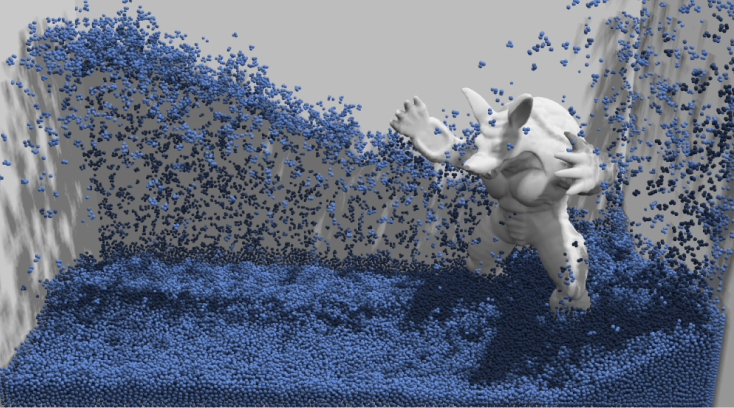
A simple position-based fluid method
Core idea:
- Assume water consists of small rigid spheres
- Assume water is incompressible (i.e. constant density)
- Whenever the density changes somewhere, “correct” it by changing particle positions
- You need the gradient of density with respect to each particle’s position
- Update method: gradient descent
Eulerian vs Lagrangian methods
There are two different viewpoints for simulating large amounts of matter, and a photography analogy makes them clear:
| Method | Alias | Core idea | Analogy |
|---|---|---|---|
| Lagrangian | Particle method | Follow the motion of each particle | A photographer follows one bird through its whole journey |
| Eulerian | Grid method | Watch the field change on a fixed grid | A photographer stands still and shoots every bird passing a given frame |
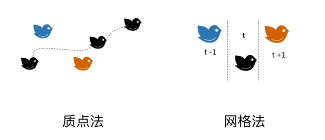
Lagrangian methods:
- Simulate the motion of each particle (point mass)
- Naturally track material boundaries
- Good for particle systems, SPH and so on
Eulerian methods:
- Observe physical quantities (density, velocity, …) on a fixed grid
- Good for grid-based fluid solvers (such as the Stable Fluids method)
- Do not track specific material; they focus on the field in space
One sentence summarises the trade-off: Lagrangian methods naturally know “where the water surface is” (you just draw where the particles are), but the particles scatter and it is hard to keep the sampling uniform; Eulerian methods naturally guarantee a uniform grid and easy differentiation, but require extra interface tracking (e.g. level sets) to know where a free surface is.
Smoothed particle hydrodynamics (SPH)
SPH is a Lagrangian method:
- Represent the fluid with particles
- Each particle carries mass, density, velocity, etc.
- Smoothly interpolate particle attributes with a kernel function
- Solve the fluid equations (a discretised form of the Navier-Stokes equations)
Advantages: handles free surfaces naturally, and parallelises well.
The Stable Fluids method
Stable Fluids is an Eulerian method, proposed by Jos Stam:
- Solve the fluid equations on a fixed grid
- Use a semi-Lagrangian scheme for advection
- Unconditionally stable (no divergence at any time step size)
- Widely used in games and visual effects
The material point method (MPM)
MPM is a hybrid method combining the Eulerian and Lagrangian viewpoints:
| Stage | Method | Operation |
|---|---|---|
| 1. Particles to grid | Lagrangian | Particles carry material attributes; transfer them to the grid |
| 2. Grid update | Eulerian | Numerically integrate on the grid |
| 3. Grid to particles | Interpolation | Interpolate the updated attributes back to the particles |
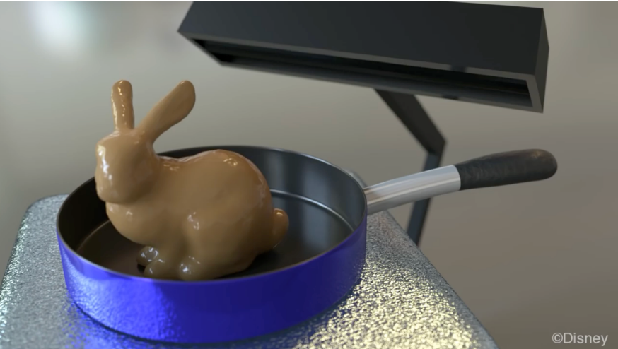
Applications: simulation of complex materials such as snow, sand and elastic bodies. The snow in Disney’s Frozen is based on this method.
(Incidentally, this shuttle of “particles carry the material → move to the grid to integrate → move back to the particles” is exactly what lets it inherit the strengths of both approaches: particles remember “what material this is” and handle topological change naturally, while the grid provides a stable numerical environment that is easy to differentiate in.)
Summary
This post covers the full spectrum from “a human describing motion” to “a computer deriving motion”, and can be reviewed along two threads.
By “who is responsible for the motion”:
| Layer | Method | Human supplies | Computer supplies |
|---|---|---|---|
| Descriptive | Keyframe animation | Keyframes and tangents | Interpolated in-between frames |
| Descriptive | Forward kinematics | Joint angles | End-effector position |
| Descriptive | Inverse kinematics | End-effector position | Joint angles |
| Data-driven | Motion capture / blend shapes | Real performance / expression bases | Retargeting and blending |
| Derivative | Mass-spring / particle systems | Forces and constraints | Motion by integration |
| Derivative | Rigid body / fluid simulation | Physical laws | Numerical solutions |
By “numerical integration” (the technical core of this post):
- Explicit Euler: simplest, first-order, prone to instability
- Midpoint / modified Euler: average the slopes, a clear improvement
- Adaptive step size: use an error estimate to adapt $\Delta t$ dynamically
- Implicit Euler: first-order but unconditionally stable, at the cost of solving a nonlinear equation
- RK4: fourth-order accuracy, the sweet spot of accuracy and stability
- Verlet / position-based: trade physical accuracy for stability via constraints and energy dissipation
One conclusion runs through the whole post: in animation, “looking right” is often more important than “computing exactly”. Whether Verlet deliberately dissipates energy or MPM shuttles between two viewpoints, each trades physical accuracy for stability and controllability. That also explains why graphics favours implicit and position-based methods, while scientific computing favours high-order explicit ones.
Post 12 notes