- Instructor: Lingqi Yan | UCSB
- Bilibili: https://www.bilibili.com/video/BV1X7411F744
- Lectures covered: Lecture 18 (Advanced Topics in Rendering)
Note: this closes out the rendering block. We walked from the rendering equation all the way to path tracing and got the basic framework standing. This post derives no new equation — it spreads out sideways instead. First, what other light transport algorithms exist (BDPT, MLT, photon mapping, VCM, instant radiosity); then, what to do when the “surface + BRDF” assumption stops being enough, and we have to model participating media, hair, skin and cloth.
1 Biased vs Unbiased
Ray tracing continues, and when it comes to rendering, everyone has their own understanding and methodology. The first question to ask about any rendering algorithm is whether its estimate is unbiased:
| Type | Definition | Characteristics |
|---|---|---|
| Unbiased | The expected value of the estimate equals the true value, regardless of the sample count | No systematic error |
| Biased | The expected value of the estimate does not equal the true value | Systematic error present |
| Consistent | Biased, but converges to the correct value as the sample count goes to infinity | Biased yet usable |
An intuitive reading: biased = blurry, consistent = not blurry once you sample infinitely.
The relationship: unbiased always implies consistent; consistent does not imply unbiased.
2 Unbiased Light Transport Methods
Bidirectional Path Tracing (BDPT)
The idea:
- Trace sub-paths from the camera and from the light separately
- Connect the endpoints of the two sub-paths
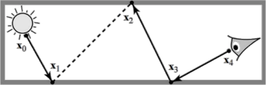
When it shines: when light transport is complicated on the light’s side.
Downside: complex to implement, and slow.
Metropolis Light Transport (MLT)
The idea: a global illumination algorithm that uses Markov Chain Monte Carlo (MCMC) sampling to find and reuse “important light paths”.
MLT’s breakthrough is that it does not sample independently — it explores the path space locally through “mutation”. Once it finds a light path that makes a significant contribution, the algorithm perturbs it slightly to produce a nearby new path; if the new path contributes more, or fits the statistics, it is “accepted”, otherwise it may be rejected. Important paths found this way get reused, which boosts sampling efficiency dramatically.
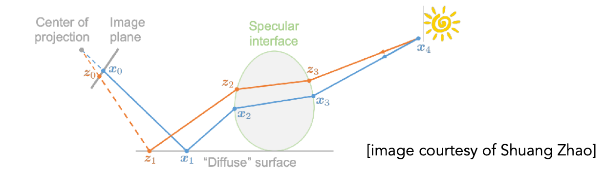
Characteristics:
- Very good at locally exploring difficult light paths
- Generates new paths by perturbing existing ones
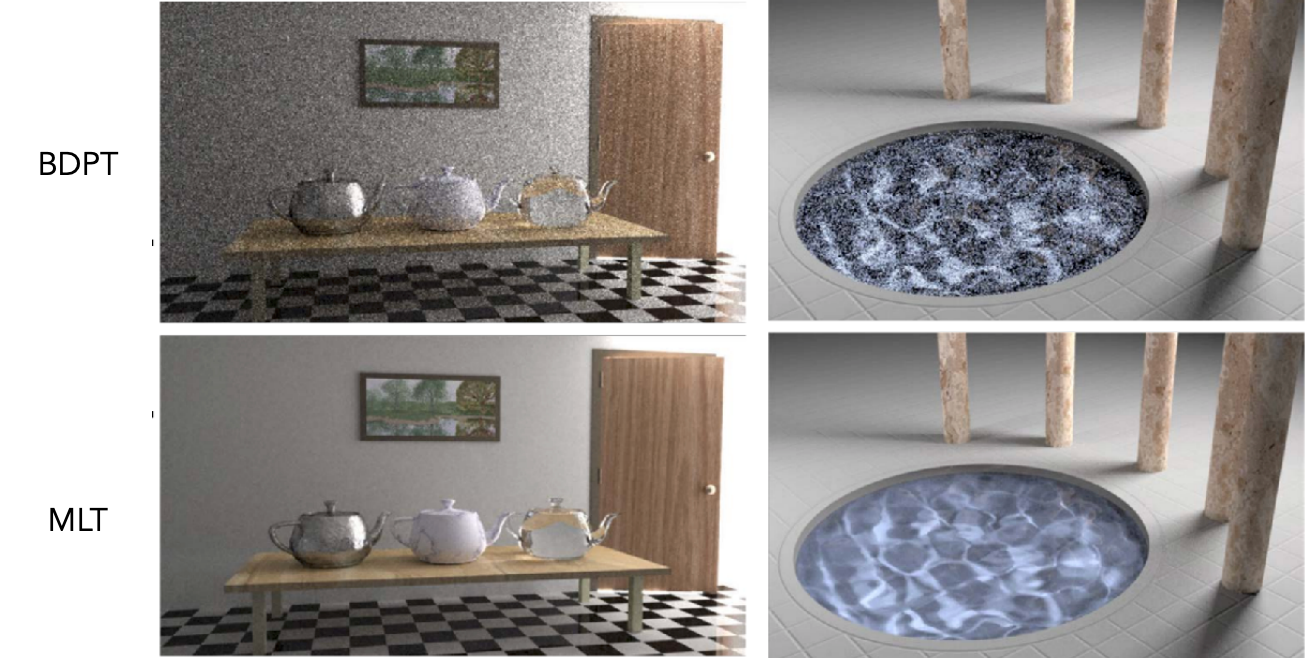
Pros: strong on difficult paths, unbiased.
Cons:
- Hard to estimate the convergence rate, hard to parallelise
- Different pixels converge at different rates, the result looks “dirty”, correlated noise lingers and needs extra cleanup
- On simple scenes it may be less efficient than path tracing or BDPT
- Unsuitable for rendering animation
3 Biased Light Transport Methods
Photon Mapping
Photon mapping is another classic global illumination algorithm, proposed by Henrik Wann Jensen in 1996. Its core idea: shoot photons out from the light, let them bounce around the scene, then collect them for rendering.
It differs from BDPT and MLT in approach: BDPT traces paths from both ends and connects them, MLT explores path space through mutation, whereas photon mapping stores light energy in the scene first, then queries it.
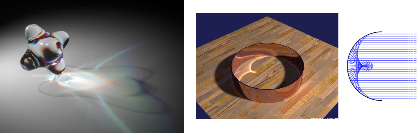
It is a two-stage method, and it is very good at handling SDS (specular-diffuse-specular) paths and producing caustics.
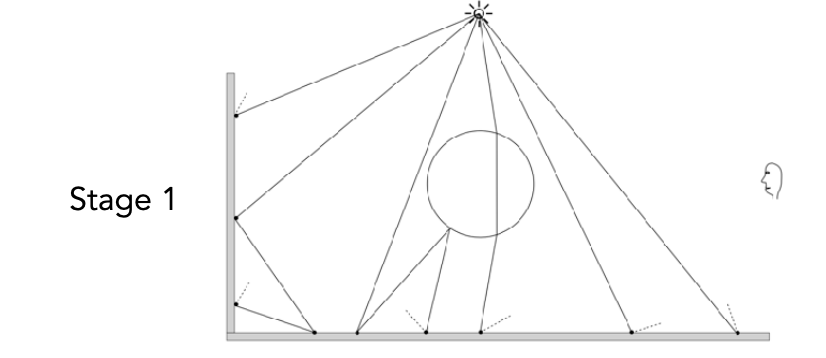
Stage 1: photon tracing
- Shoot a large number of photons from the light
- The photons travel through the scene and, on hitting a surface:
- some are absorbed
- some are reflected
- some are refracted
- Every time a photon interacts with a surface, record a photon hit point and store it in the photon map
A photon map stores: position, incident direction, energy (colour).
Stage 2: final gathering
- Shoot sub-paths from the camera that bounce onto diffuse surfaces
- Estimate illumination from the local photon density
- Add direct lighting to get the final colour
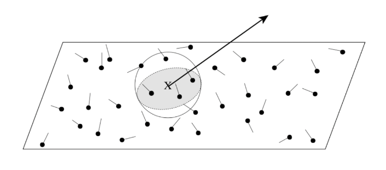
Density estimation: regions with higher photon density are brighter. For each shading point, find the nearest $N$ photons and compute the covered area $\Delta A$:
$$ \text{density} \approx \frac{\Delta N}{\Delta A} $$Why it is biased: $dN/dA \neq \Delta N / \Delta A$, but as more photons are shot, $\Delta A \to dA$, which makes it consistent.
A question from the slides: why not use a “fixed-radius search” for density estimation? — A fixed radius cannot adapt to the local photon density, and introduces bias where photons are sparse.
| Small $N$ | Large $N$ |
|---|---|
| Noisy | Blurry |
Vertex Connection and Merging (VCM)
VCM is essentially BDPT plus a “merging” sampling step. It traces paths from both the camera and the light ends, then lets each vertex contribute energy through two different strategies:
- Vertex connection: the classic BDPT operation. It tries to connect a vertex on the camera path directly to a vertex on the light path and evaluate the direct lighting between them. This handles direct lighting and indirect diffuse well — clear paths, fast.
- Vertex merging: an idea borrowed from photon mapping. It does not connect two vertices directly; instead it searches around a vertex on the camera path for cached “light vertices” (that is, photons) and estimates the indirect illumination by density estimation. This efficiently handles paths that are extremely hard to hit by connection sampling, such as reflection caustics (SDS paths).
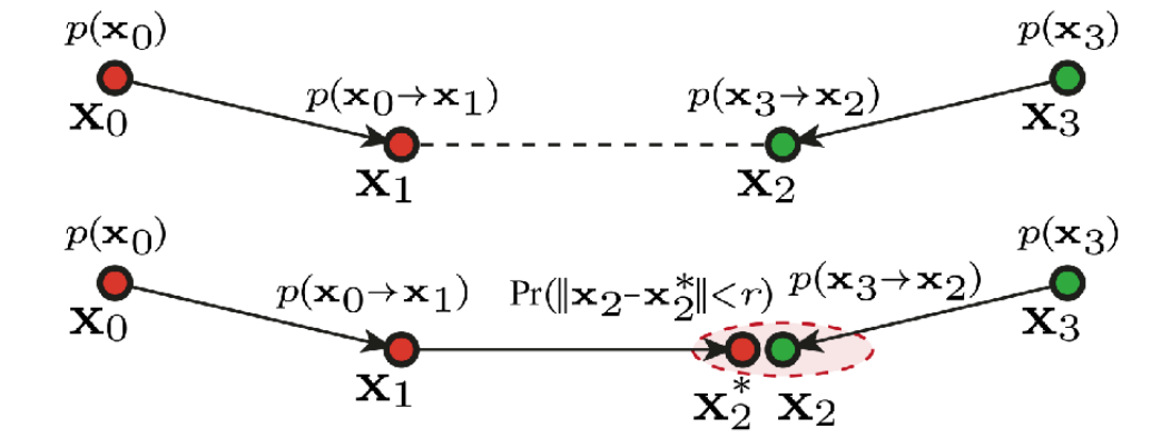
VCM’s strengths are coverage of all light path types, robustness, and automatic weighting; its weaknesses are implementation complexity, parameter sensitivity, large memory footprint, bias, and poor parallelisability. It trades complexity and bias for robustness and coverage, which suits complex offline rendering.
4 Instant Radiosity
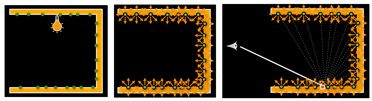
Instant Radiosity (IR) was proposed by Keller in 1997, and its core idea is very intuitive: approximate the light emitted by a source with a set of “virtual point lights”, then light the scene with those virtual lights.
Think of it as: using many tiny light bulbs to simulate the indirect illumination of a complex light source.
The method:
- Shoot sub-paths from the light, and treat the endpoint of each sub-path as a Virtual Point Light (VPL)
- Render the scene as usual with those VPLs
Pros: fast, works well for diffuse scenes.
Cons: spikes appear when a VPL gets close to a shading point, and it cannot handle glossy materials.
5 Advanced Appearance Modeling: Non-Surface Models
Non-surface models are models that interact with light without relying on the traditional notion of a “surface”. They do not deal with how an object’s surface reflects light, but with how light propagates through volumes, discrete particles, atmosphere, hair — structures that are non-continuous or non-surface.
| Model | Notes | Examples |
|---|---|---|
| Participating media | Light is absorbed and scattered in the medium; a phase function describes the scattering | Fog, clouds |
| Hair / fur | BCSDF, the glass cylinder model (Marschner), the double cylinder model | Human hair, animal fur |
| Granular material | Procedurally defined grains, avoiding explicit modelling of every grain | Sand, sugar |
6 Rendering Participating Media
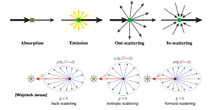
As light travels through a participating medium, it may be (partially) absorbed and scattered at any point; a phase function describes the angular distribution of scattering at any point.
Rendering steps:
- Determine the viewing path
- Sample points in the medium along the path
- At each point, compute:
- transmittance (attenuation of light from the source to that point)
- in-scattering (light from other directions scattered into the view direction)
- emission (the medium’s own glow)
- Integrate along the path, accumulating the contribution of every point
- Add the contribution of background light after attenuation through the medium
Applications: the fog in Big Hero 6 (2014) and the atmospheric effects in Assassin’s Creed Syndicate (2015).
7 Hair and Fur Appearance Models
| Model | Idea |
|---|---|
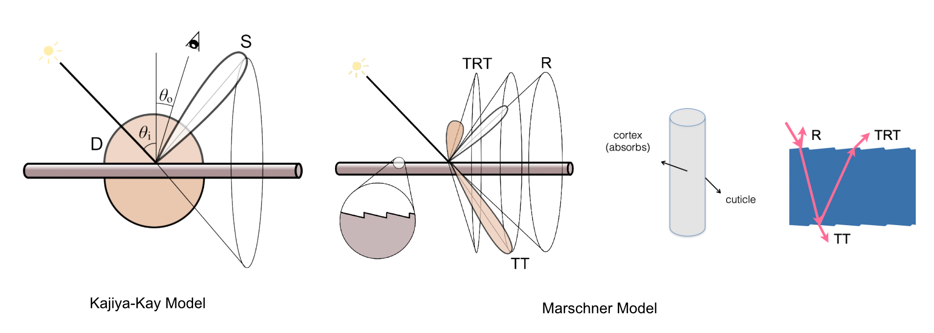
| Kajiya-Kay model | Treats hair as a matte cylinder; a tangent-based empirical reflection model |
| Marschner model | Treats hair as a glass cylinder; accurately accounts for light travelling inside the cylinder |
In the Marschner model, light interacts with hair in three ways: R (reflection), TT (transmission), TRT (internal reflection then transmission).
Hair vs Fur
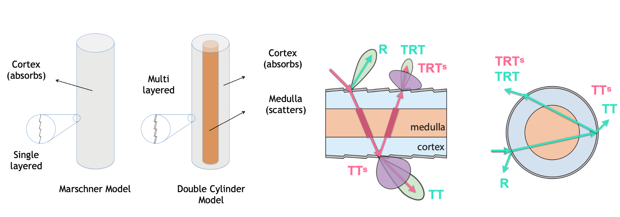
The key difference between animal fur and human hair: a fur fibre has a medulla at its core — a complex structure that scatters light. The larger the medulla, the more scattered and less saturated the appearance. Rendering fur with a human hair model fails to reproduce that diffuse, saturated look.
Double cylinder model [Yan et al. 2015, 2017]: adds a medulla layer inside the Marschner single-layer cylinder (cuticle + cortex), which produces more scattering lobes: R, TT, TRT, TTs, TRTs (the “s” denotes scattering through the medulla).
Applications: both War for the Planet of the Apes (2017) and The Lion King (2019) were nominated for the Academy Award for Best Visual Effects.
8 Granular Material
Granular material is matter made up of a large number of discrete tiny grains — sand, snow, salt, sugar, powder, soil, grain and so on.
It differs fundamentally from participating media (fog, smoke): a participating medium is continuous, whereas granular material is discrete, built from individual grains. Its rendering methods therefore borrow from participating media theory while facing their own unique challenges.

Rendering granular material means accounting both for the geometry of individual grains and for multiple scattering between grains plus light leaking through the gaps. The usual toolbox is volumetric approximation, geometric methods, hybrid methods or statistical methods — trading speed against quality.
9 Surface Models: Scattering Functions Beyond BRDF
Surface models describe how an object’s surface interacts with light — how light is reflected, refracted or scattered once it hits: from a given incoming direction onto a given point, how much energy goes out in which directions?
Mathematically, this is defined by scattering functions:
| Function | Full name | Description |
|---|---|---|
| BRDF | Bidirectional Reflectance Distribution Function | Surface reflection |
| BTDF | Bidirectional Transmittance Distribution Function | Surface transmission |
| BSDF | Bidirectional Scattering Distribution Function | BRDF + BTDF |
| BSSRDF | Bidirectional Scattering Surface Reflectance Distribution Function | Subsurface scattering |
| Model | Notes | Examples |
|---|---|---|
| Translucent material | Subsurface scattering; light enters at one point and leaves at another | Jade, jellyfish, skin |
| Cloth | Woven / knitted fibres; can be rendered as a surface, a participating medium, or actual fibres | Clothing |
| Detailed material | Non-statistical BRDF; uses normal maps to define microfacet detail | Metal glitter, scratches |
10 Subsurface Scattering
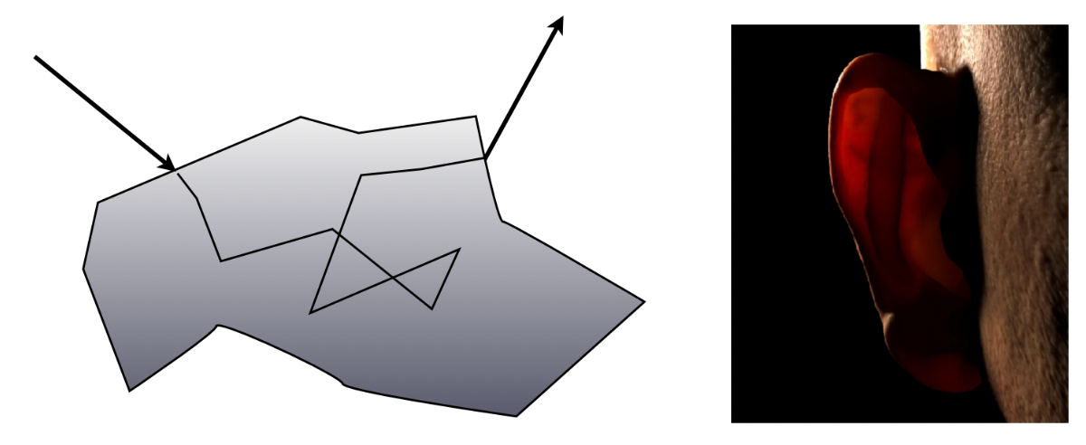
Subsurface scattering (SSS) describes the physical phenomenon where light enters a translucent material, scatters multiple times inside, and leaves through a nearby surface point.
Light enters at one surface point and exits at another after scattering inside — which violates the basic assumption of a BRDF (that the incoming and outgoing points coincide).
BSSRDF, the generalisation of the BRDF:
$$ S(x_i, \omega_i, x_o, \omega_o) $$and the corresponding rendering equation generalises to an integral over all surface points and all directions:
$$ L(x_o, \omega_o) = \int_A \int_{H^2} S(x_i, \omega_i, x_o, \omega_o) \, L_i(x_i, \omega_i) \cos\theta_i \, d\omega_i \, dA $$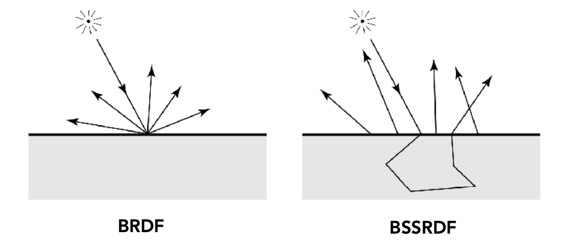
Dipole approximation [Jensen et al. 2001]: instead of solving the BSSRDF integral directly, introduce a pair of virtual point lights — one positive, one negative — below the surface of a semi-infinite medium, and use them to approximate the diffusive transport of light inside.
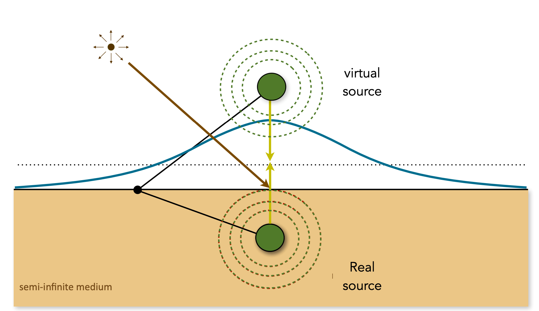
Subsurface scattering is the core reason skin, jade and milk look “translucent” and “soft”. Its mathematical model is the BSSRDF, commonly rendered via dipole, multipole, pre-integration or screen-space methods — trading speed against quality.
11 Cloth Rendering
Physical composition: cloth is fibres spun into yarn, which is then woven into fabric.
Rendering methods:
- Sheen / Charlie Sheen (simulating the soft sheen of cloth fibres)
- Ashikhmin velvet model (simulating velvet’s brighter back-lit look)
- Kajiya-Kay (an anisotropic model, simulating sheen along the yarn direction)
- Marschner hair model (multiple scattering, simulating propagation inside the fibres)
Cloth rendering has to handle fibre scattering, yarn anisotropy, weave structure, translucency and sheen — several layers of optical behaviour at once. Common models range from plain Lambert and Oren-Nayar, to dedicated Sheen, Charlie and Ashikhmin, up to physically correct path tracing with a fibre model — trading speed against quality.
12 Detailed / Glinty Material
Motivation: the NDF of a statistical microfacet model is a smooth distribution, so the render “looks too clean” compared with the real world — real car paint has glitter, real metal has scratches and smudges.
| Comparison | Statistical microfacet | Real surface |
|---|---|---|
| NDF | A smooth statistical distribution | The actual normal distribution has sharp detail |
| Normal map resolution | Typically a few thousand | Around 200K × 200K |
The difficulty: path-sampling a high-frequency normal map directly is extremely hard — in the slide example, a naive 2-hour render is nowhere near a target that needs more than 21.3 days to converge.
The solution: p-NDF (BRDF over a pixel): instead of sampling normal by normal, consider the overall NDF of the patch of normal map covered by one pixel footprint. P-NDF has sharp features, and different normal maps produce different shapes (Blender shape, brushed metal, ellipsoidal bumps, ocean waves, and so on).

Application: the glinty materials in Rise of the Tomb Raider (2016).
13 Wave Optics Appearance
The BRDF of geometric optics cannot explain diffraction: the rainbow colours of CDs, thin metal films and phone screens, or the anisotropic coloured reflections off scratched metal and the aluminium shell of a MacBook. Treating the surface as a heightfield and computing the BRDF with wave optics reproduces these effects [Yan et al. 2018].

14 Procedural Appearance
No textures needed — compute detail in real time with noise functions:
- 3D noise: when an object is cut or broken, its internal structure is there too
- Thresholding: binarise continuous noise, for example
if noise(x, y, z) > threshold:
    reflectance = 1
else:
    reflectance = 0
- Complex noise functions are remarkably powerful (Worley noise, for instance)

Summary
Lecture 18 is essentially an extension along two lines: “what else can we do with the rendering equation” and “how else can we describe a material”.
| Topic | Core content |
|---|---|
| Biased / unbiased / consistent | Unbiased means the expected value equals the true value; consistent means “biased but convergent as sampling goes to infinity”; unbiased always implies consistent, not the other way round |
| BDPT | Trace a sub-path from each of the camera and the light, then connect the endpoints; good when transport on the light side is complex, but complex to implement and slow |
| MLT | MCMC-based path mutation that reuses important paths; strong on difficult paths, but convergence is hard to estimate, hard to parallelise, and results look “dirty” |
| Photon mapping | Two stages: photon tracing into a photon map, plus final gathering and density estimation; great for SDS and caustics; biased but consistent |
| VCM | BDPT plus vertex merging; covers all path types and is robust, but complex, parameter sensitive and biased |
| Instant radiosity | Approximate a light with VPLs — “many tiny bulbs” lighting the scene; fast, but spikes near VPLs and no glossy materials |
| Non-surface models | Participating media (continuous), hair (BCSDF), granular material (discrete) |
| Participating media | Absorption and scattering in a medium; the phase function describes the angular distribution of scattering; fog, clouds |
| Hair / fur | Kajiya-Kay empirical model → Marschner glass cylinder (R/TT/TRT) → double cylinder (adds the medulla, giving TTs/TRTs) |
| Granular material | Discrete grains; must handle both grain geometry and multiple scattering plus light leaking through gaps |
| Beyond BRDF | BTDF (transmission), BSDF (reflection + transmission), BSSRDF (subsurface scattering) |
| Subsurface scattering | Light enters at one point and leaves at another; BSSRDF plus the dipole approximation; skin, jade, milk |
| Cloth | Fibre → yarn → fabric; Sheen, Charlie, Ashikhmin, Kajiya-Kay, Marschner |
| Detailed / glinty material | High-frequency normal maps are hard to sample; p-NDF represents the overall normal distribution within a pixel footprint |
| Wave optics | Diffraction and rainbow colours; treat the surface as a heightfield and compute the BRDF with wave optics |
| Procedural appearance | 3D noise plus thresholding; detail generated in real time, so a cut object is “solid all the way through” |
This post is note #9 in the GAMES101 - Modern Computer Graphics learning series.